SIC33 Production Data

Description

Statewide production data for primary metals industry (SIC 33).

Usage

data("SIC33")

Format

A data frame containing 27 observations on 3 variables.

output

Value added.

labor

Labor input.

capital

Capital stock.

Source

Online complements to Greene (2003). Table F6.1.

http://pages.stern.nyu.edu/~wgreene/Text/tables/tablelist5.htm

References

Greene, W.H. (2003). Econometric Analysis, 5th edition. Upper Saddle River, NJ: Prentice Hall.

See Also

Greene2003

Examples

data("SIC33")

## Example 6.2 in Greene (2003)
## Translog model
fm_tl <- lm(output ~ labor + capital + I(0.5 * labor^2) + I(0.5 * capital^2) + I(labor * capital),
  data = log(SIC33))
## Cobb-Douglas model
fm_cb <- lm(output ~ labor + capital, data = log(SIC33))

## Table 6.2 in Greene (2003)
deviance(fm_tl)
deviance(fm_cb)
summary(fm_tl)
summary(fm_cb)
vcov(fm_tl)
vcov(fm_cb)

## Cobb-Douglas vs. Translog model
anova(fm_cb, fm_tl)
## hypothesis of constant returns
linearHypothesis(fm_cb, "labor + capital = 1")

## 3D Visualization
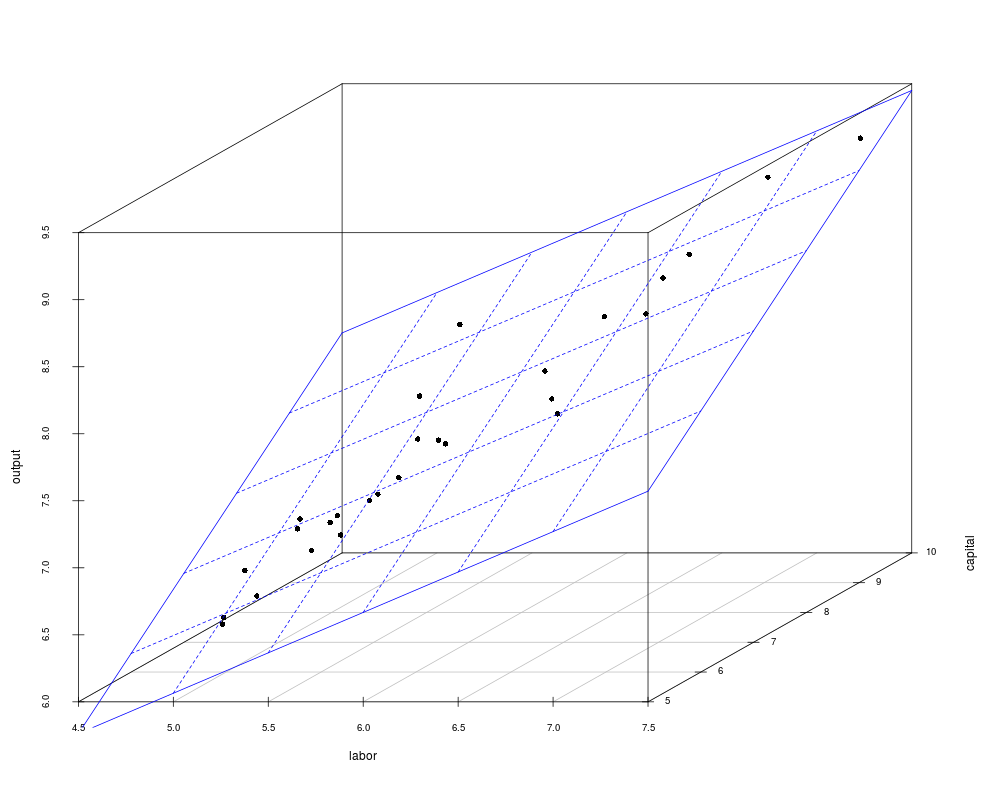
if(require("scatterplot3d")) {
  s3d <- scatterplot3d(log(SIC33)[,c(2, 3, 1)], pch = 16)
  s3d$plane3d(fm_cb, lty.box = "solid", col = 4)
}

## Interactive 3D Visualization

if(require("rgl")) {
  x <- log(SIC33)[,2]
  y <- log(SIC33)[,3]
  z <- log(SIC33)[,1]
  rgl.open()
  rgl.bbox()
  rgl.spheres(x, y, z, radius = 0.15)
  x <- seq(4.5, 7.5, by = 0.5)
  y <- seq(5.5, 10, by = 0.5)
  z <- outer(x, y, function(x, y) predict(fm_cb, data.frame(labor = x, capital = y)))
  rgl.surface(x, y, z, color = "blue", alpha = 0.5, shininess = 128)
}

Results

R version 3.3.1 (2016-06-21) -- "Bug in Your Hair"
Copyright (C) 2016 The R Foundation for Statistical Computing
Platform: x86_64-pc-linux-gnu (64-bit)

R is free software and comes with ABSOLUTELY NO WARRANTY.
You are welcome to redistribute it under certain conditions.
Type 'license()' or 'licence()' for distribution details.

R is a collaborative project with many contributors.
Type 'contributors()' for more information and
'citation()' on how to cite R or R packages in publications.

Type 'demo()' for some demos, 'help()' for on-line help, or
'help.start()' for an HTML browser interface to help.
Type 'q()' to quit R.

> library(AER)
Loading required package: car
Loading required package: lmtest
Loading required package: zoo

Attaching package: 'zoo'

The following objects are masked from 'package:base':

    as.Date, as.Date.numeric

Loading required package: sandwich
Loading required package: survival
> png(filename="/home/ddbj/snapshot/RGM3/R_CC/result/AER/SIC33.Rd_%03d_medium.png", width=480, height=480)
> ### Name: SIC33
> ### Title: SIC33 Production Data
> ### Aliases: SIC33
> ### Keywords: datasets
> 
> ### ** Examples
> 
> data("SIC33")
> 
> ## Example 6.2 in Greene (2003)
> ## Translog model
> fm_tl <- lm(output ~ labor + capital + I(0.5 * labor^2) + I(0.5 * capital^2) + I(labor * capital),
+   data = log(SIC33))
> ## Cobb-Douglas model
> fm_cb <- lm(output ~ labor + capital, data = log(SIC33))
> 
> ## Table 6.2 in Greene (2003)
> deviance(fm_tl)
[1] 0.6799272
> deviance(fm_cb)
[1] 0.8516337
> summary(fm_tl)

Call:
lm(formula = output ~ labor + capital + I(0.5 * labor^2) + I(0.5 * 
    capital^2) + I(labor * capital), data = log(SIC33))

Residuals:
     Min       1Q   Median       3Q      Max 
-0.33990 -0.10106 -0.01238  0.04605  0.39281 

Coefficients:
                   Estimate Std. Error t value Pr(>|t|)  
(Intercept)         0.94420    2.91075   0.324   0.7489  
labor               3.61364    1.54807   2.334   0.0296 *
capital            -1.89311    1.01626  -1.863   0.0765 .
I(0.5 * labor^2)   -0.96405    0.70738  -1.363   0.1874  
I(0.5 * capital^2)  0.08529    0.29261   0.291   0.7735  
I(labor * capital)  0.31239    0.43893   0.712   0.4845  
---
Signif. codes:  0 '***' 0.001 '**' 0.01 '*' 0.05 '.' 0.1 ' ' 1

Residual standard error: 0.1799 on 21 degrees of freedom
Multiple R-squared:  0.9549,	Adjusted R-squared:  0.9441 
F-statistic: 88.85 on 5 and 21 DF,  p-value: 2.121e-13

> summary(fm_cb)

Call:
lm(formula = output ~ labor + capital, data = log(SIC33))

Residuals:
     Min       1Q   Median       3Q      Max 
-0.30385 -0.10119 -0.01819  0.05582  0.50559 

Coefficients:
            Estimate Std. Error t value Pr(>|t|)    
(Intercept)  1.17064    0.32678   3.582  0.00150 ** 
labor        0.60300    0.12595   4.787 7.13e-05 ***
capital      0.37571    0.08535   4.402  0.00019 ***
---
Signif. codes:  0 '***' 0.001 '**' 0.01 '*' 0.05 '.' 0.1 ' ' 1

Residual standard error: 0.1884 on 24 degrees of freedom
Multiple R-squared:  0.9435,	Adjusted R-squared:  0.9388 
F-statistic: 200.2 on 2 and 24 DF,  p-value: 1.067e-15

> vcov(fm_tl)
                   (Intercept)       labor     capital I(0.5 * labor^2)
(Intercept)         8.47248687 -2.38790338 -0.33129294      -0.08760011
labor              -2.38790338  2.39652901 -1.23101576      -0.66580411
capital            -0.33129294 -1.23101576  1.03278652       0.52305244
I(0.5 * labor^2)   -0.08760011 -0.66580411  0.52305244       0.50039330
I(0.5 * capital^2) -0.23317345  0.03476689  0.02636926       0.14674300
I(labor * capital)  0.36354446  0.18311307 -0.22554189      -0.28803386
                   I(0.5 * capital^2) I(labor * capital)
(Intercept)               -0.23317345          0.3635445
labor                      0.03476689          0.1831131
capital                    0.02636926         -0.2255419
I(0.5 * labor^2)           0.14674300         -0.2880339
I(0.5 * capital^2)         0.08562001         -0.1160405
I(labor * capital)        -0.11604045          0.1926571
> vcov(fm_cb)
            (Intercept)        labor      capital
(Intercept)  0.10678650 -0.019835398  0.001188850
labor       -0.01983540  0.015864400 -0.009616201
capital      0.00118885 -0.009616201  0.007283931
> 
> ## Cobb-Douglas vs. Translog model
> anova(fm_cb, fm_tl)
Analysis of Variance Table

Model 1: output ~ labor + capital
Model 2: output ~ labor + capital + I(0.5 * labor^2) + I(0.5 * capital^2) + 
    I(labor * capital)
  Res.Df     RSS Df Sum of Sq      F Pr(>F)
1     24 0.85163                           
2     21 0.67993  3   0.17171 1.7678 0.1841
> ## hypothesis of constant returns
> linearHypothesis(fm_cb, "labor + capital = 1")
Linear hypothesis test

Hypothesis:
labor  + capital = 1

Model 1: restricted model
Model 2: output ~ labor + capital

  Res.Df     RSS Df Sum of Sq      F Pr(>F)
1     25 0.85574                           
2     24 0.85163  1 0.0041075 0.1158 0.7366
> 
> ## 3D Visualization
> if(require("scatterplot3d")) {
+   s3d <- scatterplot3d(log(SIC33)[,c(2, 3, 1)], pch = 16)
+   s3d$plane3d(fm_cb, lty.box = "solid", col = 4)
+ }
Loading required package: scatterplot3d
> 
> ## Interactive 3D Visualization
> ## No test: 
> if(require("rgl")) {
+   x <- log(SIC33)[,2]
+   y <- log(SIC33)[,3]
+   z <- log(SIC33)[,1]
+   rgl.open()
+   rgl.bbox()
+   rgl.spheres(x, y, z, radius = 0.15)
+   x <- seq(4.5, 7.5, by = 0.5)
+   y <- seq(5.5, 10, by = 0.5)
+   z <- outer(x, y, function(x, y) predict(fm_cb, data.frame(labor = x, capital = y)))
+   rgl.surface(x, y, z, color = "blue", alpha = 0.5, shininess = 128)
+ }
Loading required package: rgl
> ## End(No test)
> 
> 
> 
> 
> 
> dev.off()
null device 
          1 
>