R Graphical Manual

Browse All

Last data update: 2014.03.03

R: US Gasoline Market Data (1960-1995, Greene)

USGasG

R Documentation

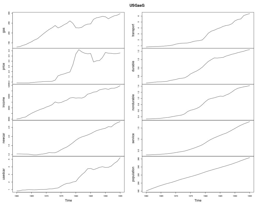
US Gasoline Market Data (1960–1995, Greene)

Description

Time series data on the US gasoline market.

Usage

data("USGasG")

Format

An annual multiple time series from 1960 to 1995 with 10 variables.

gas: Total US gasoline consumption (computed as total expenditure divided by price index).
price: Price index for gasoline.
income: Per capita disposable income.
newcar: Price index for new cars.
usedcar: Price index for used cars.
transport: Price index for public transportation.
durable: Aggregate price index for consumer durables.
nondurable: Aggregate price index for consumer nondurables.
service: Aggregate price index for consumer services.
population: US total population in millions.

Source

Online complements to Greene (2003). Table F2.2.

http://pages.stern.nyu.edu/~wgreene/Text/tables/tablelist5.htm

References

Greene, W.H. (2003). Econometric Analysis, 5th edition. Upper Saddle River, NJ: Prentice Hall.

Examples

data("USGasG", package = "AER")
plot(USGasG)

## Greene (2003)
## Example 2.3
fm <- lm(log(gas/population) ~ log(price) + log(income) + log(newcar) + log(usedcar),
  data = as.data.frame(USGasG))
summary(fm)

## Example 4.4
## estimates and standard errors (note different offset for intercept)
coef(fm)
sqrt(diag(vcov(fm)))
## confidence interval
confint(fm, parm = "log(income)")
## test linear hypothesis
linearHypothesis(fm, "log(income) = 1")

## Example 7.6
## re-used in Example 8.3
trend <- 1:nrow(USGasG)
shock <- factor(time(USGasG) > 1973, levels = c(FALSE, TRUE),
  labels = c("before", "after"))

## 1960-1995
fm1 <- lm(log(gas/population) ~ log(income) + log(price) + log(newcar) +
  log(usedcar) + trend, data = as.data.frame(USGasG))
summary(fm1)
## pooled
fm2 <- lm(log(gas/population) ~ shock + log(income) + log(price) + log(newcar) +
  log(usedcar) + trend, data = as.data.frame(USGasG))
summary(fm2)
## segmented
fm3 <- lm(log(gas/population) ~ shock/(log(income) + log(price) + log(newcar) +
  log(usedcar) + trend), data = as.data.frame(USGasG))
summary(fm3)

## Chow test
anova(fm3, fm1)
library("strucchange")
sctest(log(gas/population) ~ log(income) + log(price) + log(newcar) +
  log(usedcar) + trend, data = USGasG, point = c(1973, 1), type = "Chow")
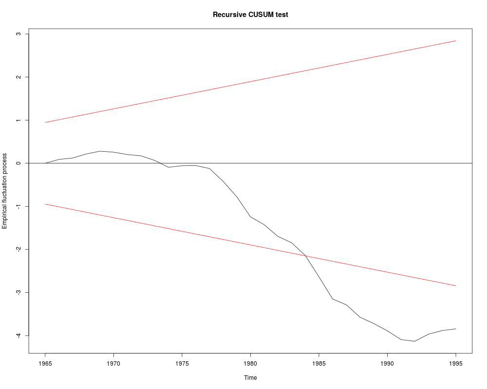
## Recursive CUSUM test
rcus <- efp(log(gas/population) ~ log(income) + log(price) + log(newcar) +
  log(usedcar) + trend, data = USGasG, type = "Rec-CUSUM")
plot(rcus)
sctest(rcus)
## Note: Greene's remark that the break is in 1984 (where the process crosses its
## boundary) is wrong. The break appears to be no later than 1976.

## More examples can be found in:
## help("Greene2003")

Results


R version 3.3.1 (2016-06-21) -- "Bug in Your Hair"
Copyright (C) 2016 The R Foundation for Statistical Computing
Platform: x86_64-pc-linux-gnu (64-bit)

R is free software and comes with ABSOLUTELY NO WARRANTY.
You are welcome to redistribute it under certain conditions.
Type 'license()' or 'licence()' for distribution details.

R is a collaborative project with many contributors.
Type 'contributors()' for more information and
'citation()' on how to cite R or R packages in publications.

Type 'demo()' for some demos, 'help()' for on-line help, or
'help.start()' for an HTML browser interface to help.
Type 'q()' to quit R.

> library(AER)
Loading required package: car
Loading required package: lmtest
Loading required package: zoo

Attaching package: 'zoo'

The following objects are masked from 'package:base':

    as.Date, as.Date.numeric

Loading required package: sandwich
Loading required package: survival
> png(filename="/home/ddbj/snapshot/RGM3/R_CC/result/AER/USGasG.Rd_%03d_medium.png", width=480, height=480)
> ### Name: USGasG
> ### Title: US Gasoline Market Data (1960-1995, Greene)
> ### Aliases: USGasG
> ### Keywords: datasets
> 
> ### ** Examples
> 
> data("USGasG", package = "AER")
> plot(USGasG)
> 
> ## Greene (2003)
> ## Example 2.3
> fm <- lm(log(gas/population) ~ log(price) + log(income) + log(newcar) + log(usedcar),
+   data = as.data.frame(USGasG))
> summary(fm)

Call:
lm(formula = log(gas/population) ~ log(price) + log(income) + 
    log(newcar) + log(usedcar), data = as.data.frame(USGasG))

Residuals:
      Min        1Q    Median        3Q       Max 
-0.065042 -0.018842  0.001528  0.020786  0.058084 

Coefficients:
              Estimate Std. Error t value Pr(>|t|)    
(Intercept)  -12.34184    0.67489 -18.287   <2e-16 ***
log(price)    -0.05910    0.03248  -1.819   0.0786 .  
log(income)    1.37340    0.07563  18.160   <2e-16 ***
log(newcar)   -0.12680    0.12699  -0.998   0.3258    
log(usedcar)  -0.11871    0.08134  -1.459   0.1545    
---
Signif. codes:  0 '***' 0.001 '**' 0.01 '*' 0.05 '.' 0.1 ' ' 1

Residual standard error: 0.03304 on 31 degrees of freedom
Multiple R-squared:  0.958,	Adjusted R-squared:  0.9526 
F-statistic: 176.7 on 4 and 31 DF,  p-value: < 2.2e-16

> 
> ## Example 4.4
> ## estimates and standard errors (note different offset for intercept)
> coef(fm)
 (Intercept)   log(price)  log(income)  log(newcar) log(usedcar) 
-12.34184054  -0.05909513   1.37339912  -0.12679667  -0.11870847 
> sqrt(diag(vcov(fm)))
 (Intercept)   log(price)  log(income)  log(newcar) log(usedcar) 
  0.67489471   0.03248496   0.07562767   0.12699351   0.08133710 
> ## confidence interval
> confint(fm, parm = "log(income)")
               2.5 %   97.5 %
log(income) 1.219155 1.527643
> ## test linear hypothesis
> linearHypothesis(fm, "log(income) = 1")
Linear hypothesis test

Hypothesis:
log(income) = 1

Model 1: restricted model
Model 2: log(gas/population) ~ log(price) + log(income) + log(newcar) + 
    log(usedcar)

  Res.Df      RSS Df Sum of Sq      F   Pr(>F)    
1     32 0.060445                                 
2     31 0.033837  1  0.026608 24.377 2.57e-05 ***
---
Signif. codes:  0 '***' 0.001 '**' 0.01 '*' 0.05 '.' 0.1 ' ' 1
> 
> ## Example 7.6
> ## re-used in Example 8.3
> trend <- 1:nrow(USGasG)
> shock <- factor(time(USGasG) > 1973, levels = c(FALSE, TRUE),
+   labels = c("before", "after"))
> 
> ## 1960-1995
> fm1 <- lm(log(gas/population) ~ log(income) + log(price) + log(newcar) +
+   log(usedcar) + trend, data = as.data.frame(USGasG))
> summary(fm1)

Call:
lm(formula = log(gas/population) ~ log(income) + log(price) + 
    log(newcar) + log(usedcar) + trend, data = as.data.frame(USGasG))

Residuals:
      Min        1Q    Median        3Q       Max 
-0.055238 -0.017715  0.003659  0.016481  0.053522 

Coefficients:
               Estimate Std. Error t value Pr(>|t|)    
(Intercept)  -17.385790   1.679289 -10.353 2.03e-11 ***
log(income)    1.954626   0.192854  10.135 3.34e-11 ***
log(price)    -0.115530   0.033479  -3.451  0.00168 ** 
log(newcar)    0.205282   0.152019   1.350  0.18700    
log(usedcar)  -0.129274   0.071412  -1.810  0.08028 .  
trend         -0.019118   0.005957  -3.210  0.00316 ** 
---
Signif. codes:  0 '***' 0.001 '**' 0.01 '*' 0.05 '.' 0.1 ' ' 1

Residual standard error: 0.02898 on 30 degrees of freedom
Multiple R-squared:  0.9687,	Adjusted R-squared:  0.9635 
F-statistic: 185.8 on 5 and 30 DF,  p-value: < 2.2e-16

> ## pooled
> fm2 <- lm(log(gas/population) ~ shock + log(income) + log(price) + log(newcar) +
+   log(usedcar) + trend, data = as.data.frame(USGasG))
> summary(fm2)

Call:
lm(formula = log(gas/population) ~ shock + log(income) + log(price) + 
    log(newcar) + log(usedcar) + trend, data = as.data.frame(USGasG))

Residuals:
      Min        1Q    Median        3Q       Max 
-0.045360 -0.019697  0.003931  0.015112  0.047550 

Coefficients:
               Estimate Std. Error t value Pr(>|t|)    
(Intercept)  -16.374402   1.456263 -11.244 4.33e-12 ***
shockafter     0.077311   0.021872   3.535  0.00139 ** 
log(income)    1.838167   0.167258  10.990 7.43e-12 ***
log(price)    -0.178005   0.033508  -5.312 1.06e-05 ***
log(newcar)    0.209842   0.129267   1.623  0.11534    
log(usedcar)  -0.128132   0.060721  -2.110  0.04359 *  
trend         -0.016862   0.005105  -3.303  0.00255 ** 
---
Signif. codes:  0 '***' 0.001 '**' 0.01 '*' 0.05 '.' 0.1 ' ' 1

Residual standard error: 0.02464 on 29 degrees of freedom
Multiple R-squared:  0.9781,	Adjusted R-squared:  0.9736 
F-statistic: 216.3 on 6 and 29 DF,  p-value: < 2.2e-16

> ## segmented
> fm3 <- lm(log(gas/population) ~ shock/(log(income) + log(price) + log(newcar) +
+   log(usedcar) + trend), data = as.data.frame(USGasG))
> summary(fm3)

Call:
lm(formula = log(gas/population) ~ shock/(log(income) + log(price) + 
    log(newcar) + log(usedcar) + trend), data = as.data.frame(USGasG))

Residuals:
      Min        1Q    Median        3Q       Max 
-0.027349 -0.006332  0.001295  0.007159  0.022016 

Coefficients:
                         Estimate Std. Error t value Pr(>|t|)    
(Intercept)              -4.13439    5.03963  -0.820 0.420075    
shockafter               -4.74111    5.51576  -0.860 0.398538    
shockbefore:log(income)   0.42400    0.57973   0.731 0.471633    
shockafter:log(income)    1.01408    0.24904   4.072 0.000439 ***
shockbefore:log(price)    0.09455    0.24804   0.381 0.706427    
shockafter:log(price)    -0.24237    0.03490  -6.946  3.5e-07 ***
shockbefore:log(newcar)   0.58390    0.21670   2.695 0.012665 *  
shockafter:log(newcar)    0.33017    0.15789   2.091 0.047277 *  
shockbefore:log(usedcar) -0.33462    0.15215  -2.199 0.037738 *  
shockafter:log(usedcar)  -0.05537    0.04426  -1.251 0.222972    
shockbefore:trend         0.02637    0.01762   1.497 0.147533    
shockafter:trend         -0.01262    0.00329  -3.835 0.000798 ***
---
Signif. codes:  0 '***' 0.001 '**' 0.01 '*' 0.05 '.' 0.1 ' ' 1

Residual standard error: 0.01488 on 24 degrees of freedom
Multiple R-squared:  0.9934,	Adjusted R-squared:  0.9904 
F-statistic: 328.5 on 11 and 24 DF,  p-value: < 2.2e-16

> 
> ## Chow test
> anova(fm3, fm1)
Analysis of Variance Table

Model 1: log(gas/population) ~ shock/(log(income) + log(price) + log(newcar) + 
    log(usedcar) + trend)
Model 2: log(gas/population) ~ log(income) + log(price) + log(newcar) + 
    log(usedcar) + trend
  Res.Df       RSS Df Sum of Sq      F    Pr(>F)    
1     24 0.0053144                                  
2     30 0.0251878 -6 -0.019873 14.958 4.595e-07 ***
---
Signif. codes:  0 '***' 0.001 '**' 0.01 '*' 0.05 '.' 0.1 ' ' 1
> library("strucchange")
> sctest(log(gas/population) ~ log(income) + log(price) + log(newcar) +
+   log(usedcar) + trend, data = USGasG, point = c(1973, 1), type = "Chow")

	Chow test

data:  log(gas/population) ~ log(income) + log(price) + log(newcar) +     log(usedcar) + trend
F = 14.958, p-value = 4.595e-07

> ## Recursive CUSUM test
> rcus <- efp(log(gas/population) ~ log(income) + log(price) + log(newcar) +
+   log(usedcar) + trend, data = USGasG, type = "Rec-CUSUM")
> plot(rcus)
> sctest(rcus)

	Recursive CUSUM test

data:  rcus
S = 1.4977, p-value = 0.0002437

> ## Note: Greene's remark that the break is in 1984 (where the process crosses its
> ## boundary) is wrong. The break appears to be no later than 1976.
> 
> ## More examples can be found in:
> ## help("Greene2003")
> 
> 
> 
> 
> 
> dev.off()
null device 
          1 
>