R Graphical Manual

Browse All

Last data update: 2014.03.03

R: Group sequential trial object (GSTobj)

GSTobj

R Documentation

Group sequential trial object (GSTobj)

Description

The GSTobj includes design and outcome of primary trial.

Usage

GSTobj(x, ...)

## S3 method for class 'GSTobj'
plot(x, main = "GSD", print.pdf = FALSE, ...)

## S3 method for class 'GSTobj'
print(x, ...)

## S3 method for class 'GSTobj'
summary(object, ctype = c("r", "so"), ptype = c("r", "so"),
  etype = c("ml", "mu", "cons"), overwrite = FALSE, ...)

## S3 method for class 'summary.GSTobj'
print(x, ...)

Arguments

`x`	object of the `class` `GSTobj`
`...`	additional arguments.
`main`	Title of the plots (default: "GSD")
`print.pdf`	option; if TRUE a pdf file is created. Instead of setting print.pdf to TRUE, the user can specify a character string giving the name or the path of the file.
`object`	object of the `class` `GSTobj`
`ctype`	confidence type: repeated "r" or stage-wise ordering "so" (default: c("r", "so"))
`ptype`	p-value type: repeated "r" or stage-wise ordering "so" (default: c("r", "so"))
`etype`	point estimate: maximum likelihood "ml", median unbiased "mu" or conservative "cons" (default: c("ml", "mu", "cons"))
`overwrite`	option; if TRUE all old values are deleted and new values are calculated (default: FALSE)

Details

A GSTobj object is designed.

The function summary returns an object of class GSTobj.

ctype defines the type of confidence interval that is calculated.

`"r"`	Repeated confidence bound for a classical GSD
`"so"`	Confidence bound for a classical GSD based on the stage-wise ordering

The calculated confidence bounds are saved as:

`cb.r`	repeated confidence bound
`cb.so`	confidence bound based on the stage-wise ordering

ptype defines the type of p-value that is calculated.

`"r"`	Repeated p-value for a classical GSD
`"so"`	Stage-wise adjusted p-value for a classical GSD

The calculated p-values are saved as:

`pvalue.r`	repeated p-value
`pvalue.so`	stage-wise adjusted p-value

etype defines the type of point estimate

`"ml"`	maximum likelihood estimate (ignoring the sequential nature of the design)
`"mu"`	median unbiased estimate (stage-wise lower confidence bound at level 0.5) for a classical GSD
`"cons"`	Conservative estimate (repeated lower confidence bound at level 0.5) for a classical GSD

The calculated point estimates are saved as:

`est.ml`	Maximum likelihood estimate
`est.mu`	Median unbiased estimate
`est.cons`	Conservative estimate

The stage-wise adjusted confidence interval and p-value and the median unbiased point estimate can only be calculated at the stage where the trial stops and is only valid if the stopping rule is met.

The repeated confidence interval and repeated p-value, conservative estimate and maximum likelihood estimate can be calculated at every stage of the trial and not just at the stage where the trial stops and is also valid if the stopping rule is not met. For calculating the repeated confidence interval or p-value at any stage of the trial the user has to specify the outcome GSDo in the object GSTobj (see example below).

Value

An object of class GSTobj, is basically a list with the elements

`cb.so`	confidence bound based on the stage-wise ordering
`cb.r`	repeated confidence bound
`pvalue.so`	stage-wise adjusted p-value
`pvalue.r`	repeated p-value
`est.ml`	maximum likelihood estimate
`est.mu`	median unbiased point estimate
`est.cons`	conservative point estimate
`GSD`
`K`	number of stages
`al`	alpha (type I error rate)
`a`	lower critical bounds of group sequential design (are currently always set to -8)
`b`	upper critical bounds of group sequential design
`t`	vector with cumulative information fraction
`SF`	spending function (for details see below)
`phi`	parameter of spending function when SF=3 or 4 (for details see below)
`alab`	alpha-absorbing parameter values of group sequential design
`als`	alpha-values ”spent” at each stage of group sequential design
`Imax`	maximum information number
`delta`	effect size used for planning the primary trial
`cp`	conditionla power of the trial
`GSDo`
`T`	stage where trial stops
`z`	z-statistic at stage where trial stops

Note

SF defines the spending function. SF = 1 O'Brien and Fleming type spending function of Lan and DeMets (1983) SF = 2 Pocock type spending function of Lan and DeMets (1983) SF = 3 Power family (c_α* t^φ). phi must be greater than 0. SF = 4 Hwang-Shih-DeCani family.(1-e^{-φ t})/(1-e^{-φ}), where phi cannot be 0. A value of SF=3 corresponds to the power family. Here, the spending function is t^{φ}, where phi must be greater than 0. A value of SF=4 corresponds to the Hwang-Shih-DeCani family, with the spending function (1-e^{-φ t})/(1-e^{-φ}), where phi cannot be 0. If a path is specified for print.pdf, all must be changed to /. If a filename is specified the ending of the file must be (.pdf). In the current version a should be set to rep(-8,K)

Author(s)

Niklas Hack niklas.hack@meduniwien.ac.at and Werner Brannath werner.brannath@meduniwien.ac.at

Examples

GSD=plan.GST(K=4,SF=1,phi=0,alpha=0.025,delta=6,pow=0.8,compute.alab=TRUE,compute.als=TRUE)
GST<-as.GST(GSD=GSD,GSDo=list(T=2, z=3.1))
GST
plot(GST)
GST<-summary(GST)
plot(GST)
##The repeated confidence interval, p-value and maximum likelihood estimate
##at the earlier stage T=1 where the trial stopping rule is not met.
summary(as.GST(GSD,GSDo=list(T=1,z=0.7)),ctype="r",ptype="r",etype="ml")
## Not run: 
##If e.g. the stage-wise adjusted confidence interval is calculated at this stage,
##the function returns an error message
summary(as.GST(GSD,GSDo=list(T=1,z=0.7)),ctype="so",etype="mu")

## End(Not run)

Results


R version 3.3.1 (2016-06-21) -- "Bug in Your Hair"
Copyright (C) 2016 The R Foundation for Statistical Computing
Platform: x86_64-pc-linux-gnu (64-bit)

R is free software and comes with ABSOLUTELY NO WARRANTY.
You are welcome to redistribute it under certain conditions.
Type 'license()' or 'licence()' for distribution details.

R is a collaborative project with many contributors.
Type 'contributors()' for more information and
'citation()' on how to cite R or R packages in publications.

Type 'demo()' for some demos, 'help()' for on-line help, or
'help.start()' for an HTML browser interface to help.
Type 'q()' to quit R.

> library(AGSDest)
> png(filename="/home/ddbj/snapshot/RGM3/R_CC/result/AGSDest/GSTobj.Rd_%03d_medium.png", width=480, height=480)
> ### Name: GSTobj
> ### Title: Group sequential trial object (GSTobj)
> ### Aliases: GSTobj plot.GSTobj print.GSTobj print.summary.GSTobj
> ###   summary.GSTobj
> ### Keywords: datasets
> 
> ### ** Examples
> 
> GSD=plan.GST(K=4,SF=1,phi=0,alpha=0.025,delta=6,pow=0.8,compute.alab=TRUE,compute.als=TRUE)
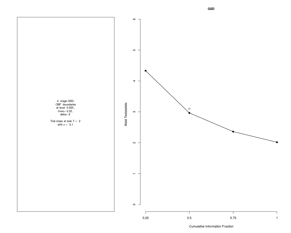
> GST<-as.GST(GSD=GSD,GSDo=list(T=2, z=3.1))
> GST
4  stage group sequential design
 alpha :  0.025   SF:  1   phi:  0   Imax:  0.22   delta:  6   cp:  0.8
                                                
Upper bounds          4.333  2.963  2.359  2.014
Lower bounds         -8.000 -8.000 -8.000 -8.000
Information fraction  0.250  0.500  0.750  1.000
                             
als   0.000 0.002 0.010 0.025
alab 10.065 3.008 0.936 0.000


group sequential design outcome:

	T:  2   z:  3.1 

> plot(GST)
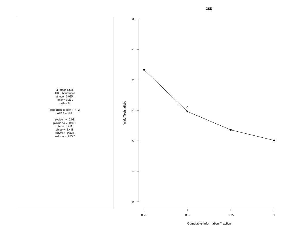
> GST<-summary(GST)
> plot(GST)
> ##The repeated confidence interval, p-value and maximum likelihood estimate
> ##at the earlier stage T=1 where the trial stopping rule is not met.
> summary(as.GST(GSD,GSDo=list(T=1,z=0.7)),ctype="r",ptype="r",etype="ml")
repeated lower confidence bound:  -15.409 

repeated p-value:  0.558 

maximum likelihood estimate:  2.969 

4  stage group sequential design
 alpha :  0.025   SF:  1   phi:  0   Imax:  0.22   delta:  6   cp:  0.8
                                                
Upper bounds          4.333  2.963  2.359  2.014
Lower bounds         -8.000 -8.000 -8.000 -8.000
Information fraction  0.250  0.500  0.750  1.000
                             
als   0.000 0.002 0.010 0.025
alab 10.065 3.008 0.936 0.000


group sequential design outcome:

	T:  1   z:  0.7 

> ## Not run: 
> ##D ##If e.g. the stage-wise adjusted confidence interval is calculated at this stage,
> ##D ##the function returns an error message
> ##D summary(as.GST(GSD,GSDo=list(T=1,z=0.7)),ctype="so",etype="mu")
> ## End(Not run)
> 
> 
> 
> 
> 
> dev.off()
null device 
          1 
>