Insect counts of 12 Species

Description

Simulated data, inpired by a real field investigating the potential impact of genetically modified crop on several insect species belonging to the same order. The trial was designed as a randomized complete block design with 8 blocks (Block), and a total of 24 plots. In each block, three treatments (Treatment) were randomized: a conventional variety treated with insecticides (Ins), a genetically modified variety (GM) without insecticide treatment, and the near-isogenic variety (Iso) the to genetically modified variety, without insecticide treatment. Individuals were counted (after classification to the species level) in two different dates in each year of the trial, where the the second date was of higher importance for assessment of impacts of GM variety on non-target species. In total 12 Species were observed during the trial.

Usage

data(Lepi)

Format

A data frame with 144 observations on the following 17 variables.

Year

a numeric vector, the year 1, 2, 3

Date

a numeric vector, 1 and 2 separating the 2 sampling date in each year

Block

a numeric vector, with values 1-8, indicator variable for the 8 blocks

Treatment

a factor with three levels identifying the varieties: GM is the genetically modified variety, Ins the conventional variety with insecticide treatment and Iso the near isognic line without insecticide treatment

Plot

a factor with 24 levels, identifying the individual plots

Sp1

counts of taxon 1

Sp2

counts of taxon 2

Sp3

counts of taxon 3

Sp4

counts of taxon 4

Sp5

counts of taxon 5

Sp6

counts of taxon 6

Sp7

counts of taxon 7

Sp8

counts of taxon 8

Sp9

counts of taxon 9

Sp10

counts of taxon 10

Sp11

counts of taxon 11

Sp12

counts of taxon 12

Source

Simulated data.

Examples

data(Lepi)

str(Lepi)

summary(Lepi)

SPEC<-names(Lepi)[-(1:5)]

# Occurrence

occur<-lapply(X=Lepi[,SPEC], FUN=function(x){length(which(x>0))})

unlist(occur)

# Species with reasonable occurence in the whole data:

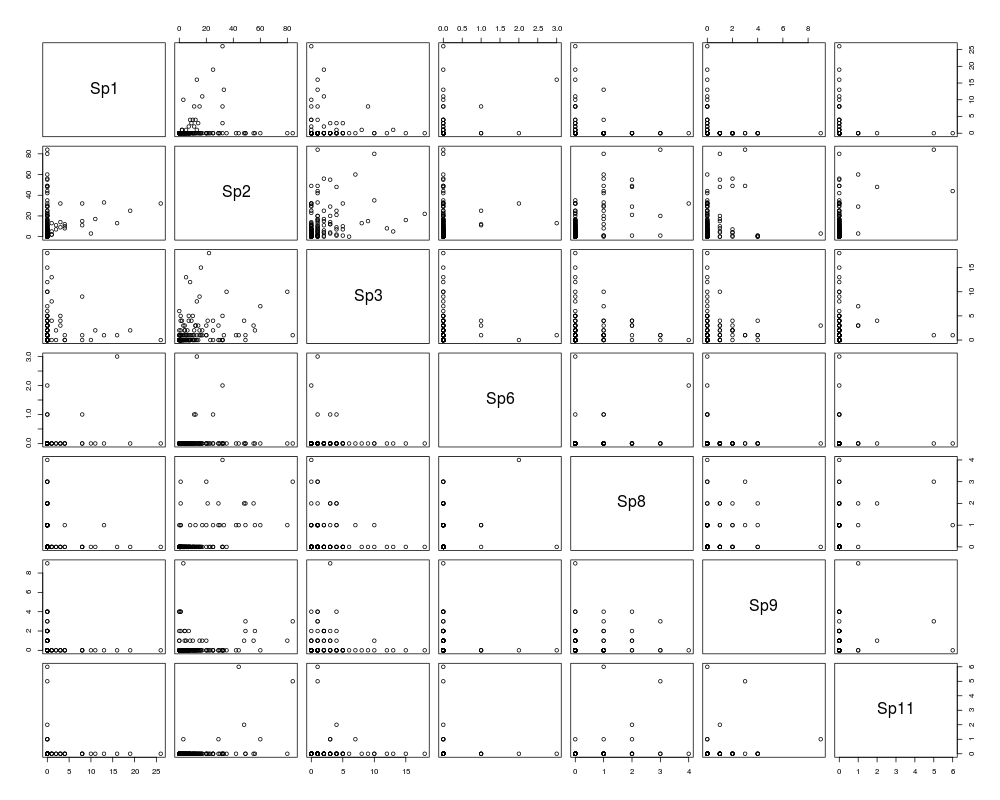
SPEC2<-SPEC[c(1,2,3,6,8,9,11)]

pairs(Lepi[,SPEC2])

# 


layout(matrix(1:2, ncol=1 ))
par(mar=c(2,8,2,1))

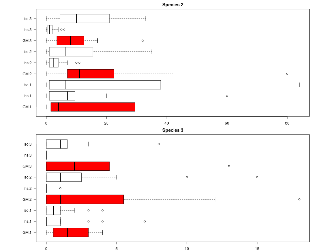
boxplot(Sp2 ~ Treatment*Year, data=Lepi, main="Species 2",
 las=1, horizontal=TRUE, col=c("red","white","white"))

boxplot(Sp3 ~ Treatment*Year, data=Lepi, main="Species 3",
 las=1, horizontal=TRUE, col=c("red","white","white"))

Results

R version 3.3.1 (2016-06-21) -- "Bug in Your Hair"
Copyright (C) 2016 The R Foundation for Statistical Computing
Platform: x86_64-pc-linux-gnu (64-bit)

R is free software and comes with ABSOLUTELY NO WARRANTY.
You are welcome to redistribute it under certain conditions.
Type 'license()' or 'licence()' for distribution details.

R is a collaborative project with many contributors.
Type 'contributors()' for more information and
'citation()' on how to cite R or R packages in publications.

Type 'demo()' for some demos, 'help()' for on-line help, or
'help.start()' for an HTML browser interface to help.
Type 'q()' to quit R.

> library(BSagri)
Loading required package: gamlss
Loading required package: splines
Loading required package: gamlss.data
Loading required package: gamlss.dist
Loading required package: MASS
Loading required package: nlme
Loading required package: parallel
 **********   GAMLSS Version 4.4-0  ********** 
For more on GAMLSS look at http://www.gamlss.org/
Type gamlssNews() to see new features/changes/bug fixes.

Loading required package: multcomp
Loading required package: mvtnorm
Loading required package: survival

Attaching package: 'survival'

The following object is masked from 'package:gamlss.data':

    leukemia

Loading required package: TH.data

Attaching package: 'TH.data'

The following object is masked from 'package:MASS':

    geyser

Loading required package: MCPAN
> png(filename="/home/ddbj/snapshot/RGM3/R_CC/result/BSagri/Lepi.Rd_%03d_medium.png", width=480, height=480)
> ### Name: Lepi
> ### Title: Insect counts of 12 Species
> ### Aliases: Lepi
> ### Keywords: datasets
> 
> ### ** Examples
> 
> 
> data(Lepi)
> 
> str(Lepi)
'data.frame':	144 obs. of  17 variables:
 $ Year     : Factor w/ 3 levels "1","2","3": 1 1 1 1 1 1 1 1 1 1 ...
 $ Date     : num  1 1 1 1 1 1 1 1 1 1 ...
 $ Block    : num  1 2 3 4 5 6 7 8 1 2 ...
 $ Treatment: Factor w/ 3 levels "GM","Ins","Iso": 1 1 1 1 1 1 1 1 2 2 ...
 $ Plot     : Factor w/ 24 levels "GM1","GM2","GM3",..: 1 2 3 4 5 6 7 8 9 10 ...
 $ Sp1      : num  0 0 0 0 0 0 0 0 0 0 ...
 $ Sp2      : num  29 49 48 49 5 4 21 30 60 2 ...
 $ Sp3      : num  3 0 4 1 1 2 4 0 7 1 ...
 $ Sp4      : num  0 0 0 0 0 0 0 0 0 0 ...
 $ Sp5      : num  0 1 0 0 0 0 0 3 0 0 ...
 $ Sp6      : num  0 0 0 0 0 0 0 0 0 0 ...
 $ Sp7      : num  0 0 0 0 0 0 0 0 0 0 ...
 $ Sp8      : num  2 2 2 1 0 0 2 1 1 0 ...
 $ Sp9      : int  0 2 1 3 0 1 0 0 0 0 ...
 $ Sp10     : num  0 0 0 0 0 0 0 0 0 0 ...
 $ Sp11     : num  1 0 2 0 0 0 0 0 1 0 ...
 $ Sp12     : num  0 0 0 0 0 0 0 0 0 0 ...
> 
> summary(Lepi)
 Year        Date         Block      Treatment      Plot          Sp1        
 1:48   Min.   :1.0   Min.   :1.00   GM :48    GM1    :  6   Min.   : 0.000  
 2:48   1st Qu.:1.0   1st Qu.:2.75   Ins:48    GM2    :  6   1st Qu.: 0.000  
 3:48   Median :1.5   Median :4.50   Iso:48    GM3    :  6   Median : 0.000  
        Mean   :1.5   Mean   :4.50             GM4    :  6   Mean   : 1.028  
        3rd Qu.:2.0   3rd Qu.:6.25             GM5    :  6   3rd Qu.: 0.000  
        Max.   :2.0   Max.   :8.00             GM6    :  6   Max.   :26.000  
                                               (Other):108                   
      Sp2             Sp3             Sp4              Sp5         
 Min.   : 0.00   Min.   : 0.00   Min.   :0.0000   Min.   :0.00000  
 1st Qu.: 1.00   1st Qu.: 0.00   1st Qu.:0.0000   1st Qu.:0.00000  
 Median : 5.00   Median : 0.00   Median :0.0000   Median :0.00000  
 Mean   :11.22   Mean   : 1.59   Mean   :0.0625   Mean   :0.03472  
 3rd Qu.:14.00   3rd Qu.: 2.00   3rd Qu.:0.0000   3rd Qu.:0.00000  
 Max.   :84.00   Max.   :18.00   Max.   :9.0000   Max.   :3.00000  
                                                                   
      Sp6               Sp7               Sp8              Sp9        
 Min.   :0.00000   Min.   :0.00000   Min.   :0.0000   Min.   :0.0000  
 1st Qu.:0.00000   1st Qu.:0.00000   1st Qu.:0.0000   1st Qu.:0.0000  
 Median :0.00000   Median :0.00000   Median :0.0000   Median :0.0000  
 Mean   :0.05556   Mean   :0.01389   Mean   :0.2917   Mean   :0.3958  
 3rd Qu.:0.00000   3rd Qu.:0.00000   3rd Qu.:0.0000   3rd Qu.:0.0000  
 Max.   :3.00000   Max.   :2.00000   Max.   :4.0000   Max.   :9.0000  
                                                                      
      Sp10               Sp11             Sp12         
 Min.   :0.000000   Min.   :0.0000   Min.   :0.000000  
 1st Qu.:0.000000   1st Qu.:0.0000   1st Qu.:0.000000  
 Median :0.000000   Median :0.0000   Median :0.000000  
 Mean   :0.006944   Mean   :0.1111   Mean   :0.006944  
 3rd Qu.:0.000000   3rd Qu.:0.0000   3rd Qu.:0.000000  
 Max.   :1.000000   Max.   :6.0000   Max.   :1.000000  
                                                       
> 
> SPEC<-names(Lepi)[-(1:5)]
> 
> # Occurrence
> 
> occur<-lapply(X=Lepi[,SPEC], FUN=function(x){length(which(x>0))})
> 
> unlist(occur)
 Sp1  Sp2  Sp3  Sp4  Sp5  Sp6  Sp7  Sp8  Sp9 Sp10 Sp11 Sp12 
  21  125   68    1    3    5    1   27   26    1    6    1 
> 
> # Species with reasonable occurence in the whole data:
> 
> SPEC2<-SPEC[c(1,2,3,6,8,9,11)]
> 
> pairs(Lepi[,SPEC2])
> 
> # 
> 
> 
> layout(matrix(1:2, ncol=1 ))
> par(mar=c(2,8,2,1))
> 
> boxplot(Sp2 ~ Treatment*Year, data=Lepi, main="Species 2",
+  las=1, horizontal=TRUE, col=c("red","white","white"))
> 
> boxplot(Sp3 ~ Treatment*Year, data=Lepi, main="Species 3",
+  las=1, horizontal=TRUE, col=c("red","white","white"))
> 
> 
> 
> 
> 
> 
> 
> dev.off()
null device 
          1 
>