Supported by Dr. Osamu Ogasawara and  . . |
|
Last data update: 2014.03.03 |
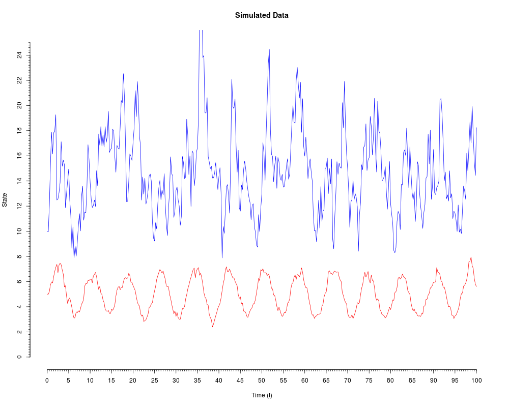
A Simulated Non-Linear Bivariate Diffusion With Time-Inhomogeneous CoefficientsDescriptionThe dataset contains discretely sampled observations for a simulated stochastic differential equation (SDE) with dynamics: dX_t = (1.0(7.5-X_t)+1.5Y_t)dt+0.5sqrt(X_tY_t)dW_t dY_t = (1.5(5-Y_t)+3sin(0.25 pi t ))dt+0.25sqrt(Y_t)dB_t where Usagedata("SDEsim4")
FormatA data frame with 401 observations on the following 3 variables.
Examplesdata(SDEsim4) attach(SDEsim4) # Have a look at the time series: plot(Xt~time,type='l',col='blue',ylim=c(0,25),main='Simulated Data', xlab='Time (t)',ylab='State',axes=FALSE) lines(Yt~time,col='red') axis(1,seq(0,100,5)) axis(1,seq(0,100,5/10),tcl=-0.2,labels=NA) axis(2,seq(0,25,2)) axis(2,seq(0,25,2/10),tcl=-0.2,labels=NA) Results
R version 3.3.1 (2016-06-21) -- "Bug in Your Hair"
Copyright (C) 2016 The R Foundation for Statistical Computing
Platform: x86_64-pc-linux-gnu (64-bit)

R is free software and comes with ABSOLUTELY NO WARRANTY.
You are welcome to redistribute it under certain conditions.
Type 'license()' or 'licence()' for distribution details.

R is a collaborative project with many contributors.
Type 'contributors()' for more information and
'citation()' on how to cite R or R packages in publications.

Type 'demo()' for some demos, 'help()' for on-line help, or
'help.start()' for an HTML browser interface to help.
Type 'q()' to quit R.

> library(DiffusionRgqd)
> png(filename="/home/ddbj/snapshot/RGM3/R_CC/result/DiffusionRgqd/SDEsim4.Rd_%03d_medium.png", width=480, height=480)
> ### Name: SDEsim4
> ### Title: A Simulated Non-Linear Bivariate Diffusion With
> ###   Time-Inhomogeneous Coefficients
> ### Aliases: SDEsim4
> ### Keywords: datasets
>
> ### ** Examples
>
> data(SDEsim4)
> attach(SDEsim4)
> # Have a look at the time series:
> plot(Xt~time,type='l',col='blue',ylim=c(0,25),main='Simulated Data',
+ xlab='Time (t)',ylab='State',axes=FALSE)
> lines(Yt~time,col='red')
> axis(1,seq(0,100,5))
> axis(1,seq(0,100,5/10),tcl=-0.2,labels=NA)
> axis(2,seq(0,25,2))
> axis(2,seq(0,25,2/10),tcl=-0.2,labels=NA)
>
>
>
>
>
>
> dev.off()
null device
          1
>
|
Created & Maintained by Osamu Ogasawara (osamu.ogasawara@gmail.com) and 