Supported by Dr. Osamu Ogasawara and  . . |
|
Last data update: 2014.03.03 |
Income Inequality in the USDescriptionData on quantiles of the distributions of family incomes in the United States. This combines three data sources: (1) US Census Table F-1 for the central quantiles (2) Piketty and Saez for the 95th and higher quantiles (3) Gross Domestic Product and implicit price deflators from MeasuringWorth.com Usagedata(incomeInequality) FormatA
DetailsFor details on how this Author(s)Spencer Graves SourceUnited States Census Bureau, Table F-1. Income Limits for Each Fifth and Top 5 Percent of Families, All Races, http://www.census.gov/hhes/www/income/data/historical/families, accessed March 25, 2014. Thomas Piketty and Emmanuel Saez (2003) "Income Inequality in the United States, 1913-1998", Quarterly Journal of Economics, 118(1) 1-39, http://elsa.berkeley.edu/~saez, update accessed February 28, 2014. Louis Johnston and Samuel H. Williamson (2011) "What Was the U.S. GDP Then?" MeasuringWorth, http://www.measuringworth.org/usgdp, accessed February 28, 2014. Examples
##
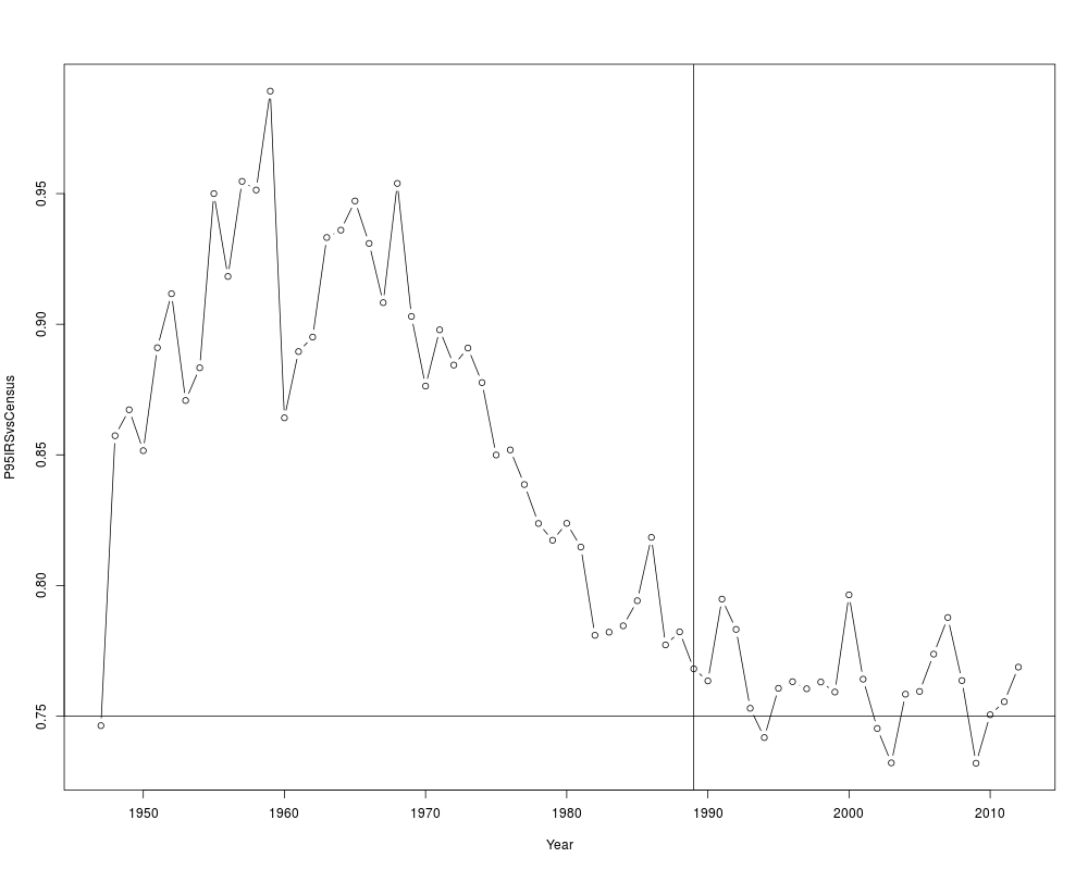
## Rato of IRS to census estimates for the 95th percentile
##
data(incomeInequality)
plot(P95IRSvsCensus~Year, incomeInequality, type='b')
# starts ~0.74, trends rapidly up to ~0.97,
# then drifts back to ~0.75
abline(h=0.75)
abline(v=1989)
# check
sum(is.na(incomeInequality$P95IRSvsCensus))
# The Census data runs to 2011; Pikety and Saez runs to 2010.
quantile(incomeInequality$P95IRSvsCensus, na.rm=TRUE)
# 0.72 ... 0.98
##
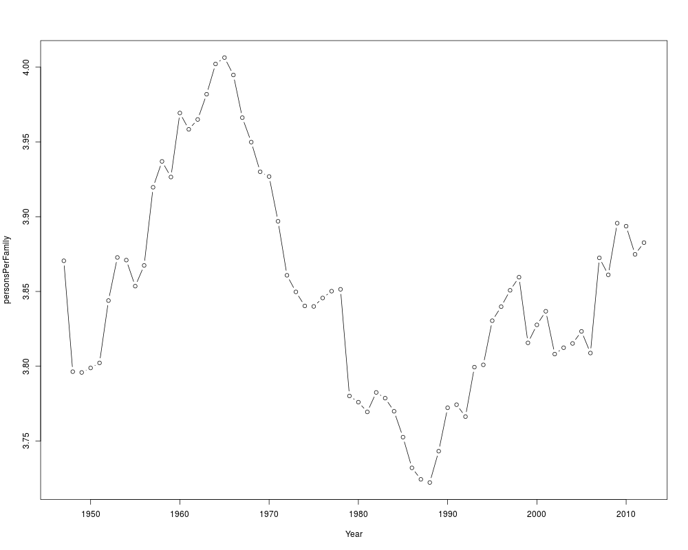
## Persons per Family
##
plot(personsPerFamily~Year, incomeInequality, type='b')
quantile(incomeInequality$personsPerFamily)
# ranges from 3.72 to 4.01 with median 3.84
# -- almost 4
##
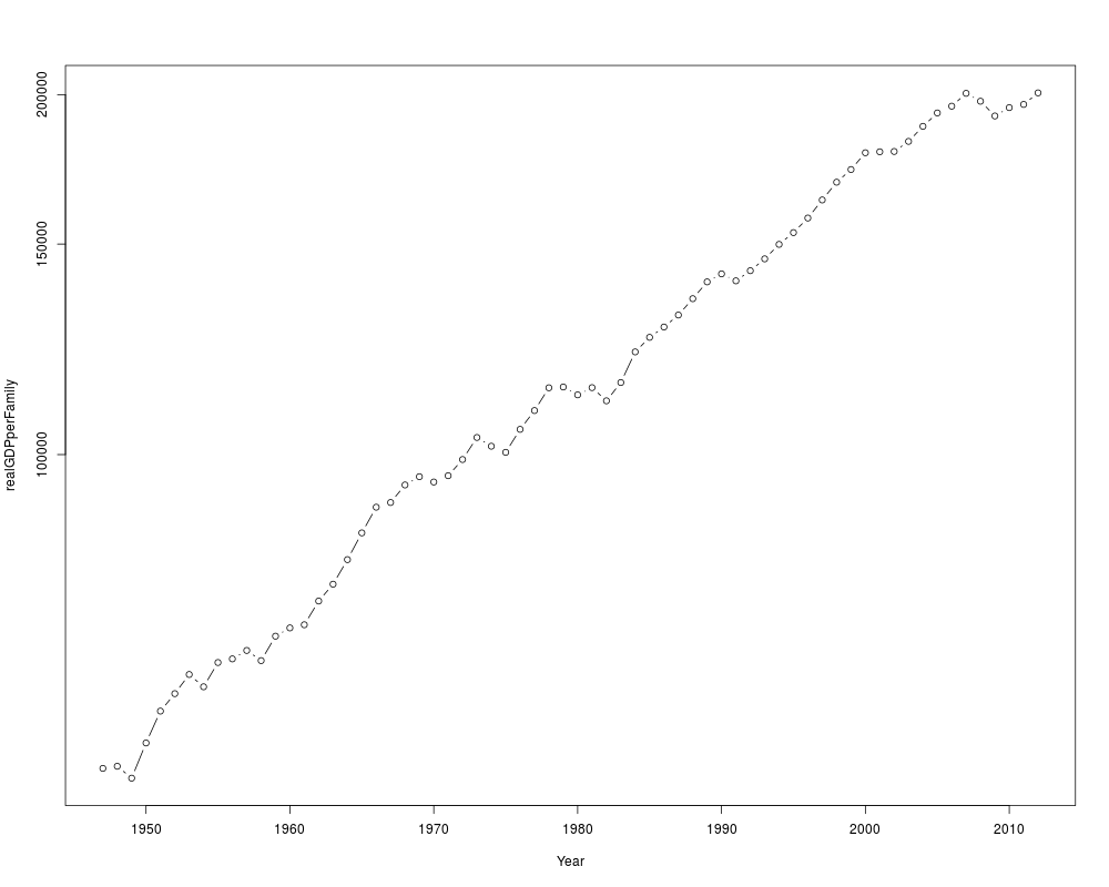
## GDP per family
##
plot(realGDPperFamily~Year, incomeInequality, type='b', log='y')
##
## Plot the mean then the first quintile, then the median,
## 99th, 99.9th and 99.99th percentiles
##
plotCols <- c(21, 3, 5, 11, 13:14)
kcols <- length(plotCols)
plotColors <- c(1:6, 8:13)[1:kcols] # omit 7=yellow
plotLty <- 1:kcols
matplot(incomeInequality$Year, incomeInequality[plotCols]/1000,
log='y', type='l', col=plotColors, lty=plotLty)
#*** Growth broadly shared 1947 - 1970, then began diverging
#*** The divergence has been most pronouced among the top 1%
#*** and especially the top 0.01%
##
## Growth rate by quantile 1947-1970 and 1970 - present
##
keyYears <- c(1947, 1970, 2010)
(iYears <- which(is.element(incomeInequality$Year, keyYears)))
(dYears <- diff(keyYears))
kk <- length(keyYears)
(lblYrs <- paste(keyYears[-kk], keyYears[-1], sep='-'))
(growth <- sapply(incomeInequality[iYears,], function(x, labels=lblYrs){
dxi <- exp(diff(log(x)))
names(dxi) <- labels
dxi
} ))
# as percent
(gr <- round(100*(growth-1), 1))
# The average annual income (realGDPperFamily) doubled between
# 1970 and 2010 (increased by 101 percent), while the median household
# income increased only 23 percent.
##
## Income lost by each quantile 1970-2010
## relative to the broadly shared growth 1947-1970
##
(lostGrowth <- (growth[, 'realGDPperFamily']-growth[, plotCols]))
# 1947-1970: The median gained 20% relative to the mean,
# while the top 1% lost ground
# 1970-2010: The median lost 79%, the 99th percentile lost 29%,
# while the top 0.1% gained
(lostIncome <- (lostGrowth[2, ] *
incomeInequality[iYears[2], plotCols]))
# The median family lost $39,000 per year in income
# relative to what they would have with the same economic growth
# broadly shared as during 1947-1970.
# That's slightly over $36,500 per year = $100 per day
(grYr <- growth^(1/dYears))
(grYr. <- round(100*(grYr-1), 1))
##
## Regression line: linear spline
##
(varyg <- c(3:14, 21))
Varyg <- names(incomeInequality)[varyg]
str(F01ps <- reshape(incomeInequality[c(1, varyg)], idvar='Year',
ids=F1.PikettySeaz$Year,
times=Varyg, timevar='pctile',
varying=list(Varyg), direction='long'))
names(F01ps)[2:3] <- c('variable', 'value')
F01ps$variable <- factor(F01ps$variable)
# linear spline basis function with knot at 1970
F01ps$t1970p <- pmax(0, F01ps$Year-1970)
table(nas <- is.na(F01ps$value))
# 6 NAs, one each of the Piketty-Saez variables in 2011
F01i <- F01ps[!nas, ]
# formula:
# log(value/1000) ~ b*Year + (for each variable:
# different intercept + (different slope after 1970))
Fit <- lm(log(value/1000)~Year+variable*t1970p, F01i)
anova(Fit)
# all highly significant
# The residuals may show problems with the model,
# but we will ignore those for now.
# Model predictions
str(Pred <- predict(Fit))
##
## Combined plot
##
# Plot to a file? Wikimedia Commons prefers svg format.
svg('incomeInequality8.svg')
# If you want software to convert svg to another format such as png,
# consider GIMP (www.gimp.org).
# Base plot
# Leave extra space on the right to label with growth since 1970
op <- par(mar=c(5, 4, 4, 5)+0.1)
matplot(incomeInequality$Year, incomeInequality[plotCols]/1000,
log='y', type='l', col=plotColors, lty=plotLty,
xlab='', ylab='', las=1, axes=FALSE, lwd=3)
axis(1, at=seq(1950, 2010, 10),
labels=c(1950, NA, 1970, NA, 1990, NA, 2010), cex.axis=1.5)
yat <- c(10, 50, 100, 500, 1000, 5000, 10000)
axis(2, yat, labels=c('$10K', '$50K', '$100K', '$500K',
'$1M', '$5M', '$10M'), las=1, cex.axis=1.2)
# Label the lines
pctls <- paste(c(20, 40, 50, 60, 80, 90, 95, 99, 99.5, 99.9, 99.99),
'%', sep='')
lineLbl0 <- c('Year', 'families K', pctls,
'realGDP.M', 'GDP deflator', 'pop-K', 'realGDPperFamily',
'95 pct(IRS / Census)', 'size of household',
'average family income', 'mean/median')
(lineLbls <- lineLbl0[plotCols])
sel75 <- (incomeInequality$Year==1975)
laby <- incomeInequality[sel75, plotCols]/1000
text(1973.5, c(1.2, 1.2, 1.3, 1.5, 1.9)*laby[-1], lineLbls[-1], cex=1.2)
text(1973.5, 1.2*laby[1], lineLbls[1], cex=1.2, srt=10)
##
## Add lines + points for the knots in 1970
##
End <- numeric(kcols)
F01names <- names(incomeInequality)
for(i in seq(length=kcols)){
seli <- (as.character(F01i$variable) == F01names[plotCols[i]])
# with(F01i[seli, ], lines(Year, exp(Pred[seli]), col=plotColors[i]))
yri <- F01i$Year[seli]
predi <- exp(Pred[seli])
lines(yri, predi, col=plotColors[i])
End[i] <- predi[length(predi)]
sel70i <- (yri==1970)
points(yri[sel70i], predi[sel70i], col=plotColors[i])
}
##
## label growth rates
##
table(sel70. <- (incomeInequality$Year>1969))
(lastYrs <- incomeInequality[sel70., 'Year'])
(lastYr. <- max(lastYrs)+4)
#text(lastYr., End, gR., xpd=NA)
text(lastYr., End, paste(gr[2, plotCols], '%', sep=''), xpd=NA)
text(lastYr.+7, End, paste(grYr.[2, plotCols], '%', sep=''), xpd=NA)
##
## Label the presidents
##
abline(v=c(1953, 1961, 1969, 1977, 1981, 1989, 1993, 2001, 2009))
(m99.95 <- with(incomeInequality, sqrt(P99.9*P99.99))/1000)
text(1949, 5000, 'Truman')
text(1956.8, 5000, 'Eisenhower', srt=90)
text(1963, 5000, 'Kennedy', srt=90)
text(1966.8, 5000, 'Johnson', srt=90)
text(1971, 5*m99.95[24], 'Nixon', srt=90)
text(1975, 5*m99.95[28], 'Ford', srt=90)
text(1978.5, 5*m99.95[32], 'Carter', srt=90)
text(1985.1, m99.95[38], 'Reagan' )
text(1991, 0.94*m99.95[44], 'GHW Bush', srt=90)
text(1997, m99.95[50], 'Clinton')
text(2005, 1.1*m99.95[58], 'GW Bush', srt=90)
text(2010, 1.2*m99.95[62], 'Obama', srt=90)
##
## Done
##
par(op) # reset margins
dev.off() # for plot to a file
Results
R version 3.3.1 (2016-06-21) -- "Bug in Your Hair"
Copyright (C) 2016 The R Foundation for Statistical Computing
Platform: x86_64-pc-linux-gnu (64-bit)

R is free software and comes with ABSOLUTELY NO WARRANTY.
You are welcome to redistribute it under certain conditions.
Type 'license()' or 'licence()' for distribution details.

R is a collaborative project with many contributors.
Type 'contributors()' for more information and
'citation()' on how to cite R or R packages in publications.

Type 'demo()' for some demos, 'help()' for on-line help, or
'help.start()' for an HTML browser interface to help.
Type 'q()' to quit R.

> library(Ecdat)
Loading required package: Ecfun

Attaching package: 'Ecfun'

The following object is masked from 'package:base':

    sign


Attaching package: 'Ecdat'

The following object is masked from 'package:datasets':

    Orange

> png(filename="/home/ddbj/snapshot/RGM3/R_CC/result/Ecdat/incomeInequality.Rd_%03d_medium.png", width=480, height=480)
> ### Name: incomeInequality
> ### Title: Income Inequality in the US
> ### Aliases: incomeInequality
> ### Keywords: datasets
>
> ### ** Examples
>
> ##
> ## Rato of IRS to census estimates for the 95th percentile
> ##
> data(incomeInequality)
> plot(P95IRSvsCensus~Year, incomeInequality, type='b')
> # starts ~0.74, trends rapidly up to ~0.97,
> # then drifts back to ~0.75
> abline(h=0.75)
> abline(v=1989)
> # check
> sum(is.na(incomeInequality$P95IRSvsCensus))
[1] 0
> # The Census data runs to 2011;  Pikety and Saez runs to 2010.
> quantile(incomeInequality$P95IRSvsCensus, na.rm=TRUE)
       0%       25%       50%       75%      100%
0.7319601 0.7637343 0.8178705 0.8905550 0.9892483
> # 0.72 ... 0.98
>
> ##
> ## Persons per Family
> ##
>
> plot(personsPerFamily~Year, incomeInequality, type='b')
> quantile(incomeInequality$personsPerFamily)
      0%      25%      50%      75%     100%
3.722238 3.798983 3.844766 3.890913 4.006411
> # ranges from 3.72 to 4.01 with median 3.84
> #  -- almost 4
>
> ##
> ## GDP per family
> ##
> plot(realGDPperFamily~Year, incomeInequality, type='b', log='y')
>
> ##
> ## Plot the mean then the first quintile, then the median,
> ##            99th, 99.9th and 99.99th percentiles
> ##
> plotCols <- c(21, 3, 5, 11, 13:14)
> kcols <- length(plotCols)
> plotColors <- c(1:6, 8:13)[1:kcols] # omit 7=yellow
> plotLty <- 1:kcols
>
> matplot(incomeInequality$Year, incomeInequality[plotCols]/1000,
+         log='y', type='l', col=plotColors, lty=plotLty)
>
> #*** Growth broadly shared 1947 - 1970, then began diverging
> #*** The divergence has been most pronouced among the top 1%
> #*** and especially the top 0.01%
>
> ##
> ## Growth rate by quantile 1947-1970 and 1970 - present
> ##
> keyYears <- c(1947, 1970, 2010)
> (iYears <- which(is.element(incomeInequality$Year, keyYears)))
[1]  1 24 64
>
> (dYears <- diff(keyYears))
[1] 23 40
> kk <- length(keyYears)
> (lblYrs <- paste(keyYears[-kk], keyYears[-1], sep='-'))
[1] "1947-1970" "1970-2010"
>
> (growth <- sapply(incomeInequality[iYears,], function(x, labels=lblYrs){
+     dxi <- exp(diff(log(x)))
+     names(dxi) <- labels
+     dxi
+ } ))
              Year Number.thousands quintile1 quintile2   median quintile3
1947-1970 1.011813         1.402557  1.889560  1.910242 1.911692  1.913143
1970-2010 1.020305         1.523331  1.037714  1.151304 1.226677  1.306985
          quintile4      p95      P90      P95      P99    P99.5    P99.9
1947-1970  1.853266 1.763044 2.132507 2.070092 1.597485 1.474057 1.305936
1970-2010  1.457630 1.647526 1.284014 1.410992 1.699962 1.822060 2.494717
            P99.99 realGDP.M GDP.Deflator PopulationK realGDPperCap
1947-1970 1.333545  2.434816     1.770543    1.422984      1.711064
1970-2010 3.914579  3.132755     4.431699    1.510447      2.074059
          P95IRSvsCensus personsPerFamily realGDPperFamily mean.median
1947-1970      1.1741578        1.0145644         1.735984    0.908088
1970-2010      0.8564303        0.9915421         2.056517    1.676494
>
> # as percent
> (gr <- round(100*(growth-1), 1))
          Year Number.thousands quintile1 quintile2 median quintile3 quintile4
1947-1970  1.2             40.3      89.0      91.0   91.2      91.3      85.3
1970-2010  2.0             52.3       3.8      15.1   22.7      30.7      45.8
           p95   P90   P95  P99 P99.5 P99.9 P99.99 realGDP.M GDP.Deflator
1947-1970 76.3 113.3 107.0 59.7  47.4  30.6   33.4     143.5         77.1
1970-2010 64.8  28.4  41.1 70.0  82.2 149.5  291.5     213.3        343.2
          PopulationK realGDPperCap P95IRSvsCensus personsPerFamily
1947-1970        42.3          71.1           17.4              1.5
1970-2010        51.0         107.4          -14.4             -0.8
          realGDPperFamily mean.median
1947-1970             73.6        -9.2
1970-2010            105.7        67.6
>
> # The average annual income (realGDPperFamily) doubled between
> # 1970 and 2010 (increased by 101 percent), while the median household
> # income increased only 23 percent.
>
> ##
> ## Income lost by each quantile 1970-2010
> ## relative to the broadly shared growth 1947-1970
> ##
> (lostGrowth <- (growth[, 'realGDPperFamily']-growth[, plotCols]))
          realGDPperFamily  quintile1     median       P99      P99.9
1947-1970                0 -0.1535755 -0.1757074 0.1384989  0.4300485
1970-2010                0  1.0188031  0.8298398 0.3565554 -0.4381997
              P99.99
1947-1970  0.4024393
1970-2010 -1.8580616
> # 1947-1970:  The median gained 20% relative to the mean,
> #           while the top 1% lost ground
> # 1970-2010:  The median lost 79%, the 99th percentile lost 29%,
> #           while the top 0.1% gained
>
> (lostIncome <- (lostGrowth[2, ] *
+                 incomeInequality[iYears[2], plotCols]))
   realGDPperFamily quintile1   median      P99     P99.9   P99.99
58                0  27419.05 42458.58 76561.71 -274125.4 -3926103
> # The median family lost $39,000 per year in income
> # relative to what they would have with the same economic growth
> # broadly shared as during 1947-1970.
> # That's slightly over $36,500 per year = $100 per day
>
> (grYr <- growth^(1/dYears))
              Year Number.thousands quintile1 quintile2   median quintile3
1947-1970 1.000511         1.014817  1.028053  1.028540 1.028574  1.028608
1970-2010 1.000503         1.010578  1.000926  1.003529 1.005121  1.006716
          quintile4     p95      P90      P95      P99    P99.5    P99.9
1947-1970  1.027187 1.02496 1.033474 1.032140 1.020575 1.017013 1.011673
1970-2010  1.009465 1.01256 1.006269 1.008644 1.013354 1.015112 1.023118
            P99.99 realGDP.M GDP.Deflator PopulationK realGDPperCap
1947-1970 1.012593  1.039448     1.025150    1.015455      1.023628
1970-2010 1.034706  1.028959     1.037921    1.010363      1.018405
          P95IRSvsCensus personsPerFamily realGDPperFamily mean.median
1947-1970      1.0070049        1.0006289         1.024271   0.9958169
1970-2010      0.9961329        0.9997877         1.018189   1.0130014
> (grYr. <- round(100*(grYr-1), 1))
          Year Number.thousands quintile1 quintile2 median quintile3 quintile4
1947-1970  0.1              1.5       2.8       2.9    2.9       2.9       2.7
1970-2010  0.1              1.1       0.1       0.4    0.5       0.7       0.9
          p95 P90 P95 P99 P99.5 P99.9 P99.99 realGDP.M GDP.Deflator PopulationK
1947-1970 2.5 3.3 3.2 2.1   1.7   1.2    1.3       3.9          2.5         1.5
1970-2010 1.3 0.6 0.9 1.3   1.5   2.3    3.5       2.9          3.8         1.0
          realGDPperCap P95IRSvsCensus personsPerFamily realGDPperFamily
1947-1970           2.4            0.7              0.1              2.4
1970-2010           1.8           -0.4              0.0              1.8
          mean.median
1947-1970        -0.4
1970-2010         1.3
>
> ##
> ## Regression line:  linear spline
> ##
>
> (varyg <- c(3:14, 21))
 [1]  3  4  5  6  7  8  9 10 11 12 13 14 21
> Varyg <- names(incomeInequality)[varyg]
> str(F01ps <- reshape(incomeInequality[c(1, varyg)], idvar='Year',
+                      ids=F1.PikettySeaz$Year,
+                      times=Varyg, timevar='pctile',
+                      varying=list(Varyg), direction='long'))
'data.frame':	858 obs. of  3 variables:
 $ Year     : num  1947 1948 1949 1950 1951 ...
 $ pctile   : chr  "quintile1" "quintile1" "quintile1" "quintile1" ...
 $ quintile1: num  14243 13779 13007 13829 15070 ...
 - attr(*, "reshapeLong")=List of 4
  ..$ varying:List of 1
  .. ..$ : chr  "quintile1" "quintile2" "median" "quintile3" ...
  ..$ v.names: NULL
  ..$ idvar  : chr "Year"
  ..$ timevar: chr "pctile"
> names(F01ps)[2:3] <- c('variable', 'value')
> F01ps$variable <- factor(F01ps$variable)
>
> # linear spline basis function with knot at 1970
> F01ps$t1970p <- pmax(0, F01ps$Year-1970)
>
> table(nas <- is.na(F01ps$value))

FALSE
  858
> # 6 NAs, one each of the Piketty-Saez variables in 2011
> F01i <- F01ps[!nas, ]
>
> # formula:
> # log(value/1000) ~ b*Year + (for each variable:
> #     different intercept + (different slope after 1970))
>
> Fit <- lm(log(value/1000)~Year+variable*t1970p, F01i)
> anova(Fit)
Analysis of Variance Table

Response: log(value/1000)
                 Df  Sum Sq Mean Sq  F value    Pr(>F)
Year              1   95.64  95.644 10577.68 < 2.2e-16 ***
variable         12 1456.23 121.353 13420.87 < 2.2e-16 ***
t1970p            1    2.09   2.090   231.10 < 2.2e-16 ***
variable:t1970p  12   11.73   0.978   108.15 < 2.2e-16 ***
Residuals       831    7.51   0.009
---
Signif. codes:  0 '***' 0.001 '**' 0.01 '*' 0.05 '.' 0.1 ' ' 1
> # all highly significant
> # The residuals may show problems with the model,
> # but we will ignore those for now.
>
> # Model predictions
> str(Pred <- predict(Fit))
 Named num [1:858] 2.64 2.67 2.7 2.72 2.75 ...
 - attr(*, "names")= chr [1:858] "1947.quintile1" "1948.quintile1" "1949.quintile1" "1950.quintile1" ...
>
> ##
> ## Combined plot
> ##
> #  Plot to a file?  Wikimedia Commons prefers svg format.
> svg('incomeInequality8.svg')
> #  If you want software to convert svg to another format such as png,
> #  consider GIMP (www.gimp.org).
>
> #  Base plot
>
> # Leave extra space on the right to label with growth since 1970
> op <- par(mar=c(5, 4, 4, 5)+0.1)
>
> matplot(incomeInequality$Year, incomeInequality[plotCols]/1000,
+         log='y', type='l', col=plotColors, lty=plotLty,
+         xlab='', ylab='', las=1, axes=FALSE, lwd=3)
> axis(1, at=seq(1950, 2010, 10),
+      labels=c(1950, NA, 1970, NA, 1990, NA, 2010), cex.axis=1.5)
> yat <- c(10, 50, 100, 500, 1000, 5000, 10000)
> axis(2, yat, labels=c('$10K', '$50K', '$100K', '$500K',
+              '$1M', '$5M', '$10M'), las=1, cex.axis=1.2)
>
> #  Label the lines
> pctls <- paste(c(20, 40, 50, 60, 80, 90, 95, 99, 99.5, 99.9, 99.99),
+               '%', sep='')
> lineLbl0 <- c('Year', 'families K', pctls,
+      'realGDP.M', 'GDP deflator', 'pop-K', 'realGDPperFamily',
+      '95 pct(IRS / Census)', 'size of household',
+      'average family income', 'mean/median')
> (lineLbls <- lineLbl0[plotCols])
[1] "mean/median" "20%"         "50%"         "99.5%"       "99.99%"
[6] "realGDP.M"
> sel75 <- (incomeInequality$Year==1975)
>
> laby <- incomeInequality[sel75, plotCols]/1000
>
> text(1973.5, c(1.2, 1.2, 1.3, 1.5, 1.9)*laby[-1], lineLbls[-1], cex=1.2)
> text(1973.5, 1.2*laby[1], lineLbls[1], cex=1.2, srt=10)
>
> ##
> ## Add lines + points for the knots in 1970
> ##
> End <- numeric(kcols)
> F01names <- names(incomeInequality)
> for(i in seq(length=kcols)){
+   seli <- (as.character(F01i$variable) == F01names[plotCols[i]])
+ #  with(F01i[seli, ], lines(Year, exp(Pred[seli]), col=plotColors[i]))
+   yri <- F01i$Year[seli]
+   predi <- exp(Pred[seli])
+   lines(yri, predi, col=plotColors[i])
+   End[i] <- predi[length(predi)]
+   sel70i <- (yri==1970)
+   points(yri[sel70i], predi[sel70i], col=plotColors[i])
+ }
>
> ##
> ##  label growth rates
> ##
> table(sel70. <- (incomeInequality$Year>1969))

FALSE  TRUE
   23    43
> (lastYrs <- incomeInequality[sel70., 'Year'])
 [1] 1970 1971 1972 1973 1974 1975 1976 1977 1978 1979 1980 1981 1982 1983 1984
[16] 1985 1986 1987 1988 1989 1990 1991 1992 1993 1994 1995 1996 1997 1998 1999
[31] 2000 2001 2002 2003 2004 2005 2006 2007 2008 2009 2010 2011 2012
> (lastYr. <- max(lastYrs)+4)
[1] 2016
> #text(lastYr., End, gR., xpd=NA)
> text(lastYr., End, paste(gr[2, plotCols], '%', sep=''), xpd=NA)
> text(lastYr.+7, End, paste(grYr.[2, plotCols], '%', sep=''), xpd=NA)
>
> ##
> ##  Label the presidents
> ##
> abline(v=c(1953, 1961, 1969, 1977, 1981, 1989, 1993, 2001, 2009))
> (m99.95 <- with(incomeInequality, sqrt(P99.9*P99.99))/1000)
 [1]  871.2137  922.2424  848.5531  945.8757  971.7336  880.5765  807.2338
 [8]  926.6332 1040.6987 1033.6739  956.3776  948.8742 1083.6977 1032.1129
[15] 1177.9390 1063.9234 1071.9227 1180.6443 1290.6369 1283.6370 1449.8320
[22] 1634.0489 1479.0661 1149.7130 1234.6856 1347.6211 1249.7151 1205.5715
[29] 1046.2963 1085.2276 1138.7454 1141.4491 1455.8189 1424.5070 1455.4575
[36] 1635.7588 1777.3875 1952.8700 2163.5463 3007.4595 1945.9916 2691.9634
[43] 2404.1387 2311.9702 2042.5027 2348.6435 2212.3710 2261.3654 2518.4364
[50] 2932.0779 3443.3017 3949.2213 4393.0757 4906.7193 3653.5077 3130.6405
[57] 3240.6360 4003.5007 4779.4529 5095.1143 5375.0219 4197.7265 3158.4421
[64] 3592.8788 3584.4502 4421.4100
>
> text(1949, 5000, 'Truman')
> text(1956.8, 5000, 'Eisenhower', srt=90)
> text(1963, 5000, 'Kennedy', srt=90)
> text(1966.8, 5000, 'Johnson', srt=90)
> text(1971, 5*m99.95[24], 'Nixon', srt=90)
> text(1975, 5*m99.95[28], 'Ford', srt=90)
> text(1978.5, 5*m99.95[32], 'Carter', srt=90)
> text(1985.1, m99.95[38], 'Reagan' )
> text(1991, 0.94*m99.95[44], 'GHW Bush', srt=90)
> text(1997, m99.95[50], 'Clinton')
> text(2005, 1.1*m99.95[58], 'GW Bush', srt=90)
> text(2010, 1.2*m99.95[62], 'Obama', srt=90)
> ##
> ##  Done
> ##
> par(op) # reset margins
>
> dev.off() # for plot to a file
png
  2
>
>
>
>
>
> dev.off()
null device
          1
>
|