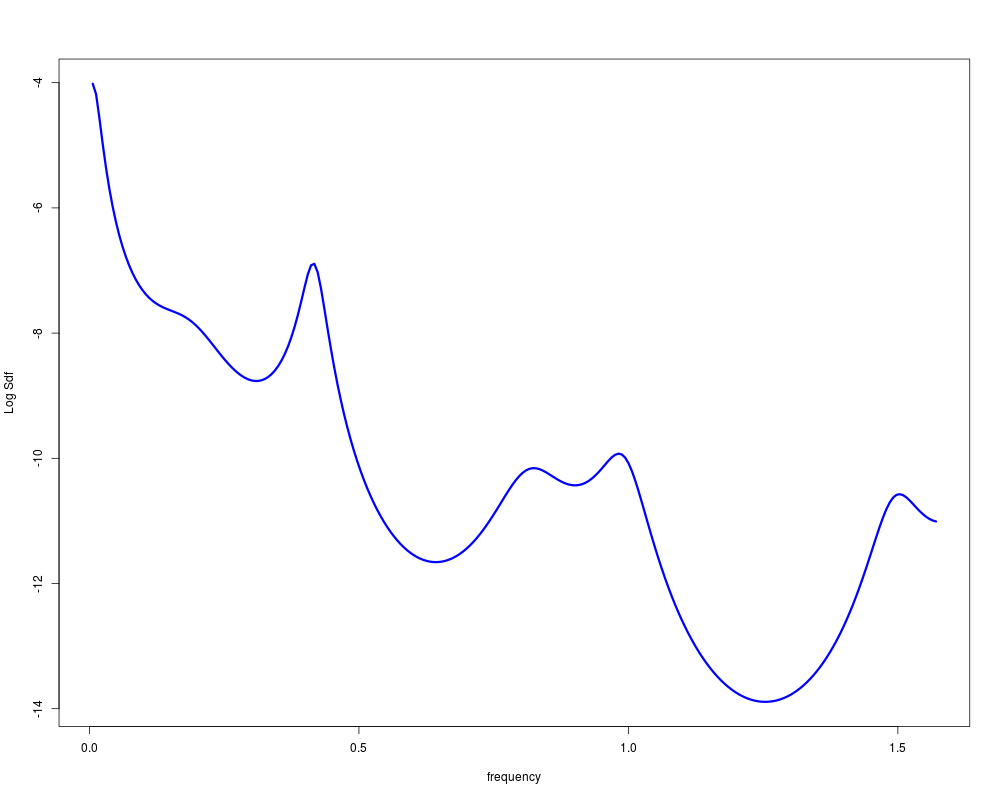
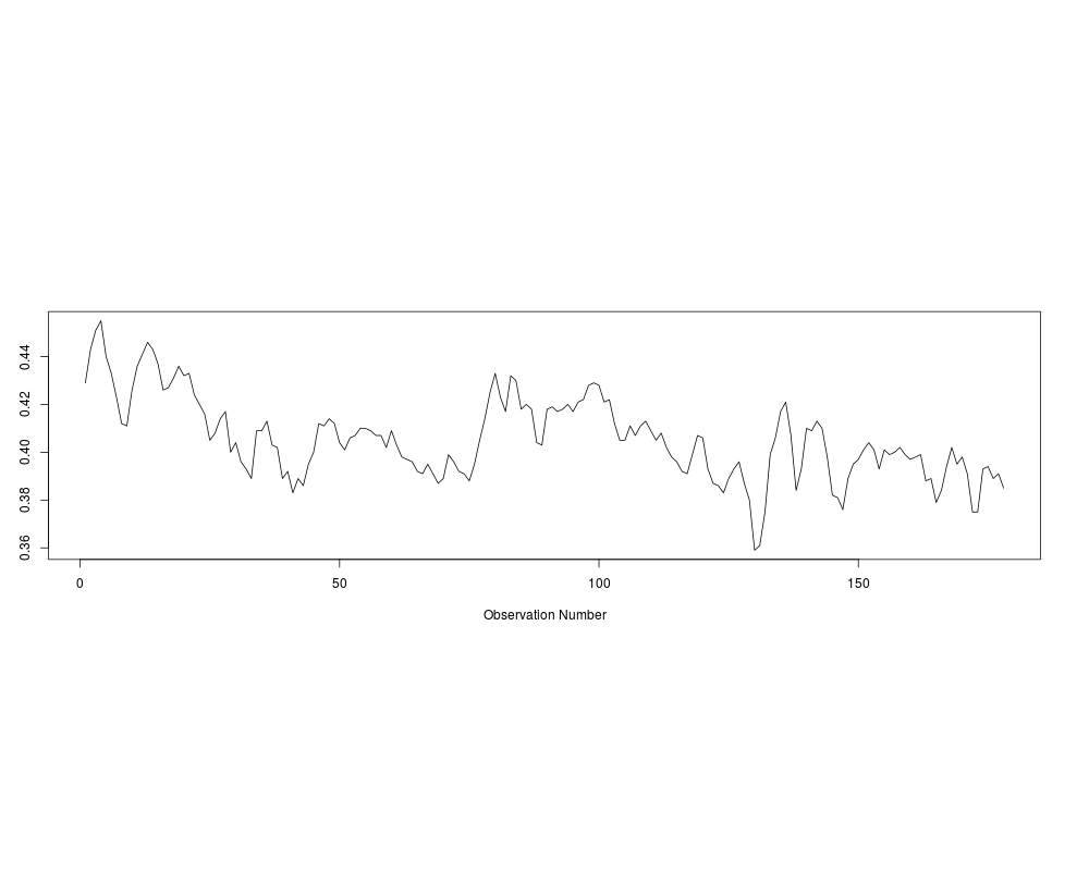
Caffeine industrial time series

Description

Hamilton and Watts (1978) state this series is produced from a cyclic industrial process with a period of 5.

Usage

data(Caffeine)

Format

The format is: num [1:178] 0.429 0.443 0.451 0.455 0.44 0.433 0.423 0.412 0.411 0.426 ...

Details

The dataset are from the paper by Hamilton and Watts (1978, Table 1). The series is used to illustrate how a multiplicative seasonal ARMA model may be identified using the partial autocorrelations. Chatfield (1979) argues that the inverse autocorrelations are more effective for model identification with this example.

Source

Hamilton, David C. and Watts, Donald G. (1978). Interpreting Partial Autocorrelation Functions of Seasonal Time Series Models. Biometrika 65/1, 135-140.

References

Hamilton, David C. and Watts, Donald G. (1978). Interpreting Partial Autocorrelation Functions of Seasonal Time Series Models. Biometrika 65/1, 135-140.

Chatfield, C. (1979). Inverse Autocorrelations. Journal of the Royal Statistical Society. Series A (General) 142/3, 363–377.

Examples

#Example 1
sdfplot(Caffeine)
TimeSeriesPlot(Caffeine)
#
#Example 2
a<-numeric(3)
names(a)<-c("AIC", "BIC", paste(sep="","BIC(q=", paste(sep="",c(0.85),")")))
z<-Caffeine
lag.max <- ceiling(length(z)/4)
a[1]<-SelectModel(z, lag.max=lag.max, ARModel="AR", Best=1, Criterion="AIC")
a[2]<-SelectModel(z, lag.max=lag.max, ARModel="AR", Best=1, Criterion="BIC")
a[3]<-SelectModel(z, lag.max=lag.max, ARModel="AR", Best=1, Criterion="BICq", t=0.85)
a

Results

R version 3.3.1 (2016-06-21) -- "Bug in Your Hair"
Copyright (C) 2016 The R Foundation for Statistical Computing
Platform: x86_64-pc-linux-gnu (64-bit)

R is free software and comes with ABSOLUTELY NO WARRANTY.
You are welcome to redistribute it under certain conditions.
Type 'license()' or 'licence()' for distribution details.

R is a collaborative project with many contributors.
Type 'contributors()' for more information and
'citation()' on how to cite R or R packages in publications.

Type 'demo()' for some demos, 'help()' for on-line help, or
'help.start()' for an HTML browser interface to help.
Type 'q()' to quit R.

> library(FitAR)
Loading required package: lattice
Loading required package: leaps
Loading required package: ltsa
Loading required package: bestglm
> png(filename="/home/ddbj/snapshot/RGM3/R_CC/result/FitAR/Caffeine.Rd_%03d_medium.png", width=480, height=480)
> ### Name: Caffeine
> ### Title: Caffeine industrial time series
> ### Aliases: Caffeine
> ### Keywords: datasets
> 
> ### ** Examples
> 
> #Example 1
> sdfplot(Caffeine)
> TimeSeriesPlot(Caffeine)
> #
> #Example 2
> a<-numeric(3)
> names(a)<-c("AIC", "BIC", paste(sep="","BIC(q=", paste(sep="",c(0.85),")")))
> z<-Caffeine
> lag.max <- ceiling(length(z)/4)
> a[1]<-SelectModel(z, lag.max=lag.max, ARModel="AR", Best=1, Criterion="AIC")
> a[2]<-SelectModel(z, lag.max=lag.max, ARModel="AR", Best=1, Criterion="BIC")
> a[3]<-SelectModel(z, lag.max=lag.max, ARModel="AR", Best=1, Criterion="BICq", t=0.85)
> a
        AIC         BIC BIC(q=0.85) 
         18          11           7 
> 
> 
> 
> 
> 
> dev.off()
null device 
          1 
>