Soil Electrical Conductivity

Description

Electrical conductivity of soil paste extracts from the Lower Arkansas River Valley, at sites upstream and downstream of the John Martin Reservoir.

Usage

data(ArkansasRiver)

Format

The format is: List of 2 $ upstream : num [1:823] 2.37 3.53 3.06 3.35 3.07 ... $ downstream: num [1:435] 8.75 6.59 5.09 6.03 5.64 ...

Details

Electrical conductivity is a measure of soil water salinity.

Source

This data set was supplied by Eric Morway (emorway@usgs.gov).

References

Eric D. Morway and Timothy K. Gates (2011) Regional assessment of soil water salinity across an extensively irrigated river valley. Journal of Irrigation and Drainage Engineering, doi:10.1061/(ASCE)IR.1943-4774.0000411

Examples

data(ArkansasRiver)
lapply(ArkansasRiver, summary)
upstream <- ArkansasRiver[[1]]
downstream <- ArkansasRiver[[2]]
## Fit normal inverse Gaussian
## Hyperbolic can also be fitted but fit is not as good
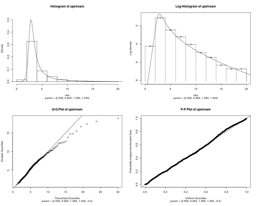
fitUpstream <- nigFit(upstream)
summary(fitUpstream)
par(mfrow = c(2,2))
plot(fitUpstream)
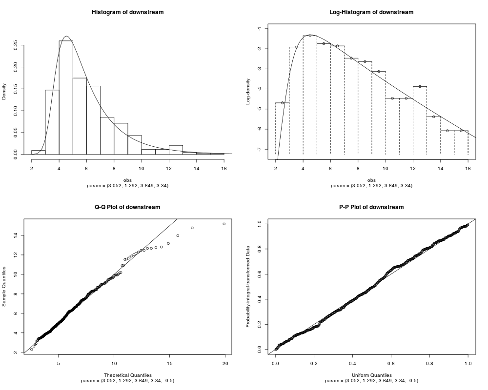
fitDownstream <- nigFit(downstream)
summary(fitDownstream)
plot(fitDownstream)
par(mfrow = c(1,1))
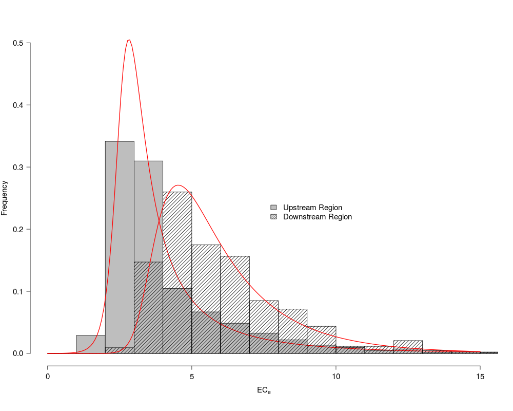
## Combined plot to compare
## Reproduces Figure 3 from Morway and Gates (2011)
hist(upstream, col = "grey", xlab = "", ylab = "", cex.axis = 1.25,
     main = "", breaks = seq(0,20, by = 1), xlim = c(0,15), las = 1,
     ylim = c(0,0.5), freq = FALSE)
param <- coef(fitUpstream)
nigDens <- function(x) dnig(x, param = param)
curve(nigDens, 0, 15, n = 201, add = TRUE,
      ylab = NULL, col = "red", lty = 1, lwd = 1.7)

hist(downstream, add = TRUE, col = "black", angle = 45, density = 15,
     breaks = seq(0,20, by = 1), freq = FALSE)
param <- coef(fitDownstream)
nigDens <- function(x) dnig(x, param = param)
curve(nigDens, 0, 15, n = 201, add = TRUE,
      ylab = NULL, col = "red", lty = 1, lwd = 1.7)

mtext(expression(EC[e]), side = 1, line = 3, cex = 1.25)
mtext("Frequency", side = 2, line = 3, cex = 1.25)
legend(x = 7.5, y = 0.250, c("Upstream Region","Downstream Region"),
       col = c("black","black"), density = c(NA,25),
       fill = c("grey","black"), angle = c(NA,45),
       cex = 1.25, bty = "n", xpd = TRUE)

Results

R version 3.3.1 (2016-06-21) -- "Bug in Your Hair"
Copyright (C) 2016 The R Foundation for Statistical Computing
Platform: x86_64-pc-linux-gnu (64-bit)

R is free software and comes with ABSOLUTELY NO WARRANTY.
You are welcome to redistribute it under certain conditions.
Type 'license()' or 'licence()' for distribution details.

R is a collaborative project with many contributors.
Type 'contributors()' for more information and
'citation()' on how to cite R or R packages in publications.

Type 'demo()' for some demos, 'help()' for on-line help, or
'help.start()' for an HTML browser interface to help.
Type 'q()' to quit R.

> library(GeneralizedHyperbolic)
Loading required package: DistributionUtils
Loading required package: RUnit
> png(filename="/home/ddbj/snapshot/RGM3/R_CC/result/GeneralizedHyperbolic/ArkansasRiver.Rd_%03d_medium.png", width=480, height=480)
> ### Name: ArkansasRiver
> ### Title: Soil Electrical Conductivity
> ### Aliases: ArkansasRiver
> ### Keywords: datasets
> 
> ### ** Examples
> 
> data(ArkansasRiver)
> lapply(ArkansasRiver, summary)
$upstream
   Min. 1st Qu.  Median    Mean 3rd Qu.    Max. 
  1.107   2.767   3.255   4.104   4.602  18.980 

$downstream
   Min. 1st Qu.  Median    Mean 3rd Qu.    Max. 
  2.296   4.360   5.361   5.986   7.009  15.180 

> upstream <- ArkansasRiver[[1]]
> downstream <- ArkansasRiver[[2]]
> ## Fit normal inverse Gaussian
> ## Hyperbolic can also be fitted but fit is not as good
> fitUpstream <- nigFit(upstream)
> summary(fitUpstream)

Data:      upstream 
Parameter estimates:
    mu   delta   alpha    beta  
2.5557  0.6616  1.5825  1.4551  
Likelihood:         -1441.33 
Method:             Nelder-Mead 
Convergence code:   0 
Iterations:         223 
> par(mfrow = c(2,2))
> plot(fitUpstream)
> fitDownstream <- nigFit(downstream)
> summary(fitDownstream)

Data:      downstream 
Parameter estimates:
   mu  delta  alpha   beta  
3.052  1.292  3.649  3.340  
Likelihood:         -880.0715 
Method:             Nelder-Mead 
Convergence code:   0 
Iterations:         293 
> plot(fitDownstream)
> par(mfrow = c(1,1))
> ## Combined plot to compare
> ## Reproduces Figure 3 from Morway and Gates (2011)
> hist(upstream, col = "grey", xlab = "", ylab = "", cex.axis = 1.25,
+      main = "", breaks = seq(0,20, by = 1), xlim = c(0,15), las = 1,
+      ylim = c(0,0.5), freq = FALSE)
> param <- coef(fitUpstream)
> nigDens <- function(x) dnig(x, param = param)
> curve(nigDens, 0, 15, n = 201, add = TRUE,
+       ylab = NULL, col = "red", lty = 1, lwd = 1.7)
> 
> hist(downstream, add = TRUE, col = "black", angle = 45, density = 15,
+      breaks = seq(0,20, by = 1), freq = FALSE)
> param <- coef(fitDownstream)
> nigDens <- function(x) dnig(x, param = param)
> curve(nigDens, 0, 15, n = 201, add = TRUE,
+       ylab = NULL, col = "red", lty = 1, lwd = 1.7)
> 
> mtext(expression(EC[e]), side = 1, line = 3, cex = 1.25)
> mtext("Frequency", side = 2, line = 3, cex = 1.25)
> legend(x = 7.5, y = 0.250, c("Upstream Region","Downstream Region"),
+        col = c("black","black"), density = c(NA,25),
+        fill = c("grey","black"), angle = c(NA,45),
+        cex = 1.25, bty = "n", xpd = TRUE)
> 
> 
> 
> 
> 
> dev.off()
null device 
          1 
>