Supported by Dr. Osamu Ogasawara and  . . |
|
Last data update: 2014.03.03 |
Elderton and Pearson's (1910) data on drinking and wagesDescriptionIn 1910, Karl Pearson weighed in on the debate, fostered by the temperance movement, on the evils done by alcohol not only to drinkers, but to their families. The report "A first study of the influence of parental alcholism on the physique and ability of their offspring" was an ambitious attempt to the new methods of statistics to bear on an important question of social policy, to see if the hypothesis that children were damaged by parental alcoholism would stand up to statistical scrutiny. Working with his assistant, Ethel M. Elderton, Pearson collected voluminous data in Edinburgh and Manchester on many aspects of health, stature, intelligence, etc. of children classified according to the drinking habits of their parents. His conclusions where almost invariably negative: the tendency of parents to drink appeared unrelated to any thing he had measured. The firestorm that this report set off is well described by Stigler (1999),
Chapter 1. The data set Usagedata(DrinksWages) FormatA data frame with 70 observations on the following 6 variables, giving the number of non-drinkers (
DetailsThe data give Karl Pearson's tabulation of the father's trades from an Edinburgh sample, classified by whether they dring or are sober, and giving average weekly wage. The wages are averages of the individuals' nominal wages. Class A is those with wages under 2.5s.; B: those with wages 2.5s. to 30s.; C: wages over 30s. SourcePearson, K. (1910). The Times, August 10, 1910. Stigler, S. M. (1999). Statistics on the Table: The History of Statistical Concepts and Methods. Harvard University Press, Table 1.1 ReferencesM. E. Elderton & K. Pearson (1910). A first study of the influence of parental alcholism on the physique and ability of their offspring, Eugenics Laboratory Memoirs, 10. Examples
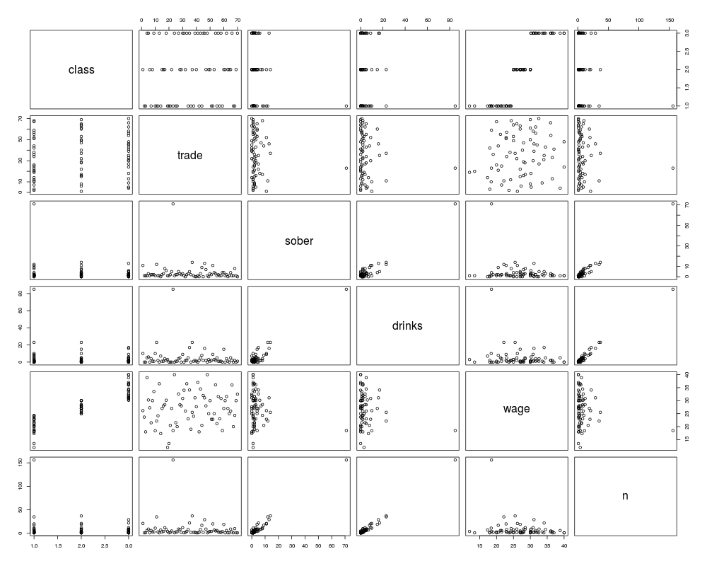
data(DrinksWages)
plot(DrinksWages)
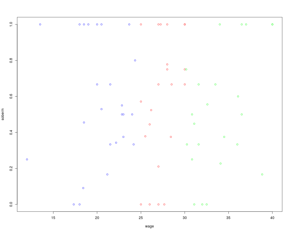
# plot proportion sober vs. wage | class
with(DrinksWages, plot(wage, sober/n, col=c("blue","red","green")[class]))
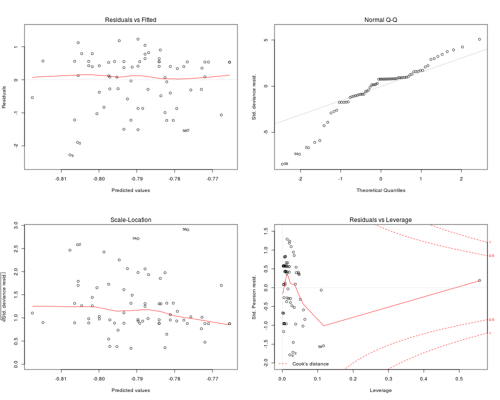
# fit logistic regression model of sober on wage
mod.sober <- glm(cbind(sober, n) ~ wage, family=binomial, data=DrinksWages)
summary(mod.sober)
op <- par(mfrow=c(2,2))
plot(mod.sober)
par(op)
# TODO: plot fitted model
Results
R version 3.3.1 (2016-06-21) -- "Bug in Your Hair"
Copyright (C) 2016 The R Foundation for Statistical Computing
Platform: x86_64-pc-linux-gnu (64-bit)

R is free software and comes with ABSOLUTELY NO WARRANTY.
You are welcome to redistribute it under certain conditions.
Type 'license()' or 'licence()' for distribution details.

R is a collaborative project with many contributors.
Type 'contributors()' for more information and
'citation()' on how to cite R or R packages in publications.

Type 'demo()' for some demos, 'help()' for on-line help, or
'help.start()' for an HTML browser interface to help.
Type 'q()' to quit R.

> library(HistData)
> png(filename="/home/ddbj/snapshot/RGM3/R_CC/result/HistData/DrinksWages.Rd_%03d_medium.png", width=480, height=480)
> ### Name: DrinksWages
> ### Title: Elderton and Pearson's (1910) data on drinking and wages
> ### Aliases: DrinksWages
> ### Keywords: datasets
>
> ### ** Examples
>
> data(DrinksWages)
> plot(DrinksWages)
>
> # plot proportion sober vs. wage | class
> with(DrinksWages, plot(wage, sober/n, col=c("blue","red","green")[class]))
>
> # fit logistic regression model of sober on wage
> mod.sober <- glm(cbind(sober, n) ~ wage, family=binomial, data=DrinksWages)
> summary(mod.sober)

Call:
glm(formula = cbind(sober, n) ~ wage, family = binomial, data = DrinksWages)

Deviance Residuals:
    Min       1Q   Median       3Q      Max
-2.2720  -0.5235   0.3472   0.5476   1.2329

Coefficients:
             Estimate Std. Error z value Pr(>|z|)
(Intercept) -0.839963   0.323962  -2.593  0.00952 **
wage         0.001862   0.012811   0.145  0.88443
---
Signif. codes:  0 '***' 0.001 '**' 0.01 '*' 0.05 '.' 0.1 ' ' 1

(Dispersion parameter for binomial family taken to be 1)

    Null deviance: 44.717  on 69  degrees of freedom
Residual deviance: 44.696  on 68  degrees of freedom
AIC: 194.06

Number of Fisher Scoring iterations: 4

> op <- par(mfrow=c(2,2))
> plot(mod.sober)
> par(op)
>
> # TODO: plot fitted model
>
>
>
>
>
> dev.off()
null device
          1
>
|