Darwin's Heights of Cross- and Self-fertilized Zea May Pairs

Description

Darwin (1876) studied the growth of pairs of zea may (aka corn) seedlings, one produced by cross-fertilization and the other produced by self-fertilization, but otherwise grown under identical conditions. His goal was to demonstrate the greater vigour of the cross-fertilized plants. The data recorded are the final height (inches, to the nearest 1/8th) of the plants in each pair.

In the Design of Experiments, Fisher (1935) used these data to illustrate a paired t-test (well, a one-sample test on the mean difference, cross - self). Later in the book (section 21), he used this data to illustrate an early example of a non-parametric permutation test, treating each paired difference as having (randomly) either a positive or negative sign.

Usage

data(ZeaMays)

Format

A data frame with 15 observations on the following 4 variables.

pair

pair number, a numeric vector

pot

pot, a factor with levels 1 2 3 4

cross

height of cross fertilized plant, a numeric vector

self

height of cross fertilized plant, a numeric vector

diff

cross - self for each pair

Details

In addition to the standard paired t-test, several types of non-parametric tests can be contemplated:

(a) Permutation test, where the values of, say self are permuted and diff=cross - self is calculated for each permutation. There are 15! permutations, but a reasonably large number of random permutations would suffice. But this doesn't take the paired samples into account.

(b) Permutation test based on assigning each abs(diff) a + or - sign, and calculating the mean(diff). There are 2^{15} such possible values. This is essentially what Fisher proposed. The p-value for the test is the proportion of absolute mean differences under such randomization which exceed the observed mean difference.

(c) Wilcoxon signed rank test: tests the hypothesis that the median signed rank of the diff is zero, or that the distribution of diff is symmetric about 0, vs. a location shifted alternative.

Source

Darwin, C. (1876). The Effect of Cross- and Self-fertilization in the Vegetable Kingdom, 2nd Ed. London: John Murray.

Andrews, D. and Herzberg, A. (1985) Data: a collection of problems from many fields for the student and research worker. New York: Springer. Data retrieved from: https://www.stat.cmu.edu/StatDat/

References

Fisher, R. A. (1935). The Design of Experiments. London: Oliver & Boyd.

See Also

wilcox.test

independence_test in the coin package, a general framework for conditional inference procedures (permutation tests)

Examples

data(ZeaMays)

##################################
## Some preliminary exploration ##
##################################
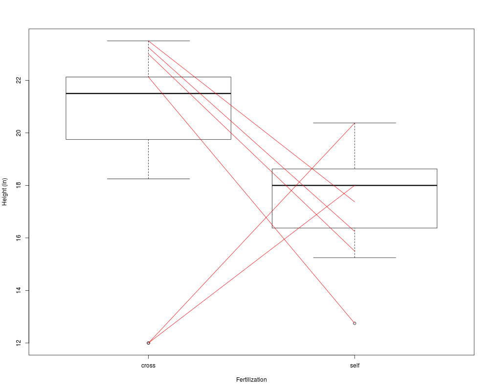
boxplot(ZeaMays[,c("cross", "self")], ylab="Height (in)", xlab="Fertilization")

# examine large individual diff/ces
largediff <- subset(ZeaMays, abs(diff) > 2*sd(abs(diff)))
with(largediff, segments(1, cross, 2, self, col="red"))

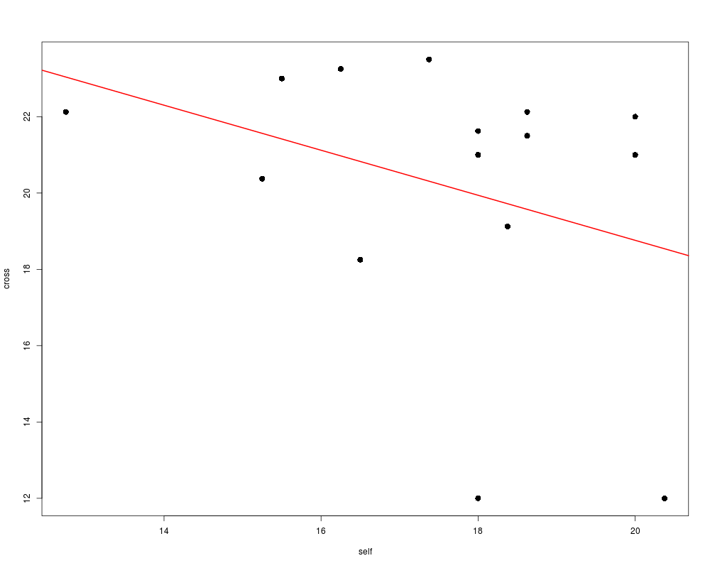
# plot cross vs. self.  NB: unusual trend and some unusual points
with(ZeaMays, plot(self, cross, pch=16, cex=1.5))
abline(lm(cross ~ self, data=ZeaMays), col="red", lwd=2)

# pot effects ?
 anova(lm(diff ~ pot, data=ZeaMays))

##############################
## Tests of mean difference ##
##############################
# Wilcoxon signed rank test
# signed ranks:
with(ZeaMays, sign(diff) * rank(abs(diff)))
wilcox.test(ZeaMays$cross, ZeaMays$self, conf.int=TRUE, exact=FALSE)

# t-tests
with(ZeaMays, t.test(cross, self))
with(ZeaMays, t.test(diff))

mean(ZeaMays$diff)
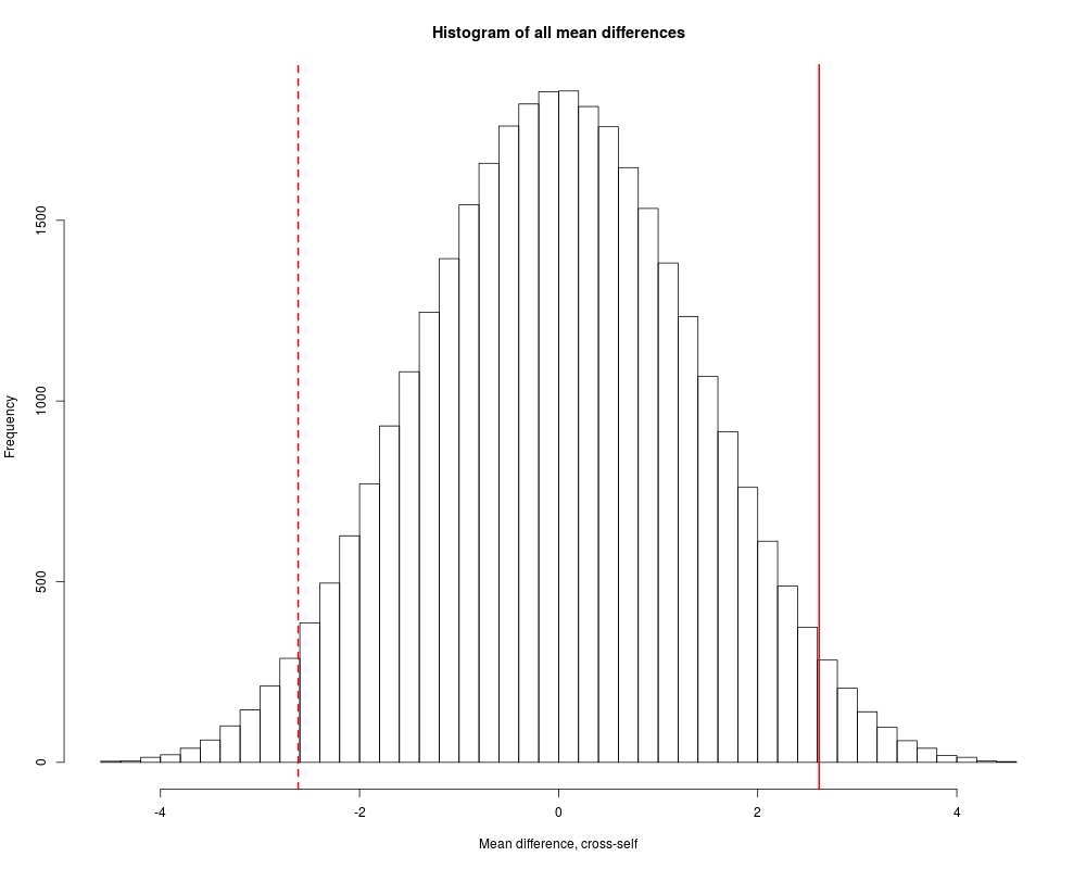
# complete permutation distribution of diff, for all 2^15 ways of assigning
# one value to cross and the other to self (thx: Bert Gunter)
N <- nrow(ZeaMays)
allmeans <- as.matrix(expand.grid(as.data.frame(
                         matrix(rep(c(-1,1),N), nr =2))))  %*% abs(ZeaMays$diff) / N

# upper-tail p-value
sum(allmeans > mean(ZeaMays$diff)) / 2^N
# two-tailed p-value
sum(abs(allmeans) > mean(ZeaMays$diff)) / 2^N

hist(allmeans, breaks=64, xlab="Mean difference, cross-self",
	main="Histogram of all mean differences")
abline(v=c(1, -1)*mean(ZeaMays$diff), col="red", lwd=2, lty=1:2)

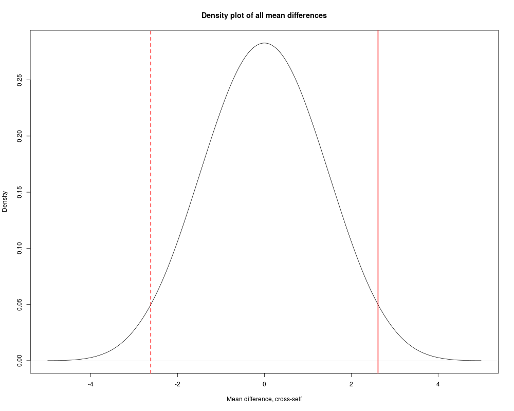
plot(density(allmeans), xlab="Mean difference, cross-self",
	main="Density plot of all mean differences")
abline(v=c(1, -1)*mean(ZeaMays$diff), col="red", lwd=2, lty=1:2)

Results

R version 3.3.1 (2016-06-21) -- "Bug in Your Hair"
Copyright (C) 2016 The R Foundation for Statistical Computing
Platform: x86_64-pc-linux-gnu (64-bit)

R is free software and comes with ABSOLUTELY NO WARRANTY.
You are welcome to redistribute it under certain conditions.
Type 'license()' or 'licence()' for distribution details.

R is a collaborative project with many contributors.
Type 'contributors()' for more information and
'citation()' on how to cite R or R packages in publications.

Type 'demo()' for some demos, 'help()' for on-line help, or
'help.start()' for an HTML browser interface to help.
Type 'q()' to quit R.

> library(HistData)
> png(filename="/home/ddbj/snapshot/RGM3/R_CC/result/HistData/ZeaMays.Rd_%03d_medium.png", width=480, height=480)
> ### Name: ZeaMays
> ### Title: Darwin's Heights of Cross- and Self-fertilized Zea May Pairs
> ### Aliases: ZeaMays
> ### Keywords: datasets nonparametric
> 
> ### ** Examples
> 
> data(ZeaMays)
> 
> ##################################
> ## Some preliminary exploration ##
> ##################################
> boxplot(ZeaMays[,c("cross", "self")], ylab="Height (in)", xlab="Fertilization")
> 
> # examine large individual diff/ces
> largediff <- subset(ZeaMays, abs(diff) > 2*sd(abs(diff)))
> with(largediff, segments(1, cross, 2, self, col="red"))
> 
> # plot cross vs. self.  NB: unusual trend and some unusual points
> with(ZeaMays, plot(self, cross, pch=16, cex=1.5))
> abline(lm(cross ~ self, data=ZeaMays), col="red", lwd=2)
> 
> # pot effects ?
>  anova(lm(diff ~ pot, data=ZeaMays))
Analysis of Variance Table

Response: diff
          Df  Sum Sq Mean Sq F value Pr(>F)
pot        3  44.692  14.898  0.6139 0.6201
Residuals 11 266.947  24.268               
> 
> ##############################
> ## Tests of mean difference ##
> ##############################
> # Wilcoxon signed rank test
> # signed ranks:
> with(ZeaMays, sign(diff) * rank(abs(diff)))
 [1]  11 -14   2   4   1   5   7   9   3   8  12   6  15  13 -10
> wilcox.test(ZeaMays$cross, ZeaMays$self, conf.int=TRUE, exact=FALSE)

	Wilcoxon rank sum test with continuity correction

data:  ZeaMays$cross and ZeaMays$self
W = 185.5, p-value = 0.002608
alternative hypothesis: true location shift is not equal to 0
95 percent confidence interval:
 1.625009 4.875007
sample estimates:
difference in location 
              3.374989 

> 
> # t-tests
> with(ZeaMays, t.test(cross, self))

	Welch Two Sample t-test

data:  cross and self
t = 2.4371, df = 22.164, p-value = 0.02328
alternative hypothesis: true difference in means is not equal to 0
95 percent confidence interval:
 0.3909566 4.8423767
sample estimates:
mean of x mean of y 
 20.19167  17.57500 

> with(ZeaMays, t.test(diff))

	One Sample t-test

data:  diff
t = 2.148, df = 14, p-value = 0.0497
alternative hypothesis: true mean is not equal to 0
95 percent confidence interval:
 0.003899165 5.229434169
sample estimates:
mean of x 
 2.616667 

> 
> mean(ZeaMays$diff)
[1] 2.616667
> # complete permutation distribution of diff, for all 2^15 ways of assigning
> # one value to cross and the other to self (thx: Bert Gunter)
> N <- nrow(ZeaMays)
> allmeans <- as.matrix(expand.grid(as.data.frame(
+                          matrix(rep(c(-1,1),N), nr =2))))  %*% abs(ZeaMays$diff) / N
> 
> # upper-tail p-value
> sum(allmeans > mean(ZeaMays$diff)) / 2^N
[1] 0.02548218
> # two-tailed p-value
> sum(abs(allmeans) > mean(ZeaMays$diff)) / 2^N
[1] 0.05096436
> 
> hist(allmeans, breaks=64, xlab="Mean difference, cross-self",
+ 	main="Histogram of all mean differences")
> abline(v=c(1, -1)*mean(ZeaMays$diff), col="red", lwd=2, lty=1:2)
> 
> plot(density(allmeans), xlab="Mean difference, cross-self",
+ 	main="Density plot of all mean differences")
> abline(v=c(1, -1)*mean(ZeaMays$diff), col="red", lwd=2, lty=1:2)
> 
> 
> 
> 
> 
> 
> 
> dev.off()
null device 
          1 
>