Salaries table

Description

Player salary data.

Usage

data(Salaries)

Format

A data frame with 23956 observations on the following 5 variables.

yearID

Year

teamID

Team; a factor

lgID

League; a factor

playerID

Player ID code

salary

Salary

Details

There is no real coverage of player's salaries until 1985.

Source

Lahman, S. (2015) Lahman's Baseball Database, 1871-2014, 2015 version, http://baseball1.com/statistics/

Examples

# what years are included?
summary(Salaries$yearID)
# how many players included each year?
table(Salaries$yearID)

# Team salary data

require(plyr)

# Total team salaries by league, team and year
teamSalaries <- ddply(Salaries, .(lgID, teamID, yearID), summarise,
                       Salary = sum(as.numeric(salary)))

# Arrange in decreasing order within year and league:
teamSalaries <- ddply(teamSalaries, .(yearID, lgID), arrange, desc(Salary))

#######################################
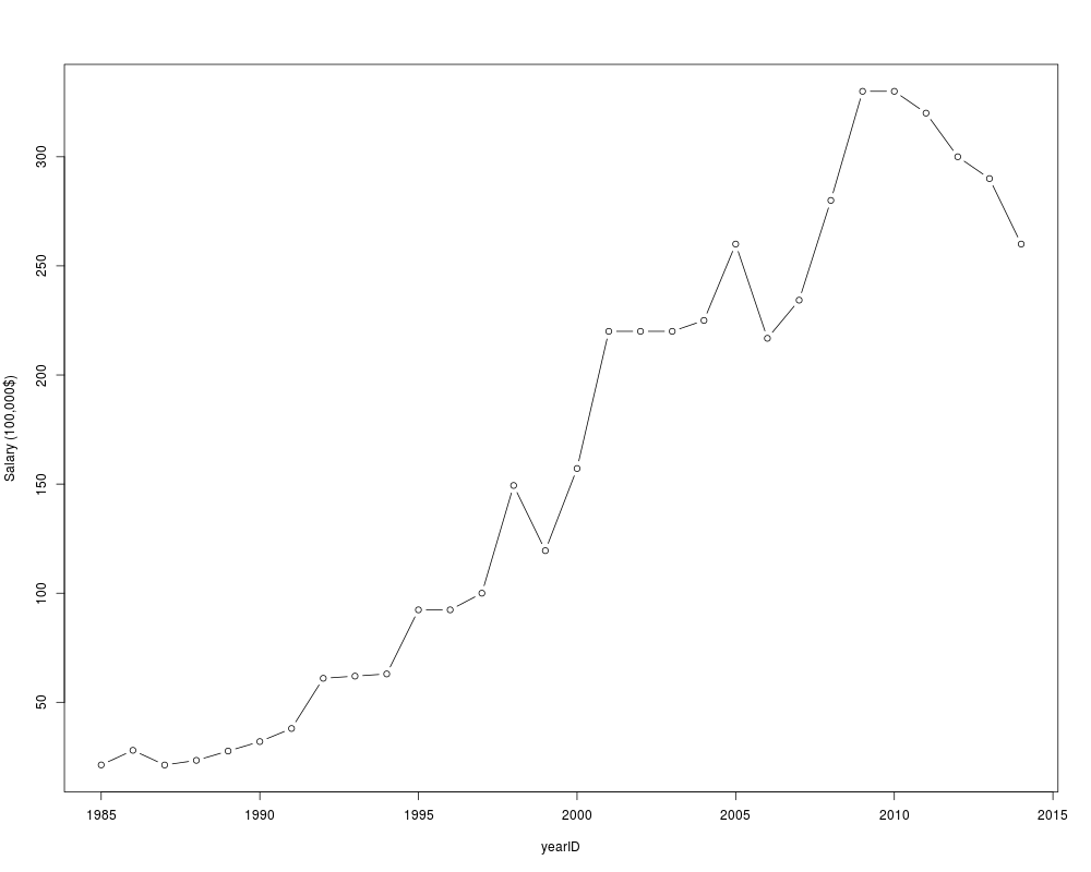
# Highest paid players each year:
maxSal <- ddply(Salaries, .(yearID), subset, salary == max(salary))
names <- apply(t(sapply(maxSal$playerID, playerInfo))[,2:3], 2, paste)
maxSal <- cbind(maxSal, names)
maxSal
plot(salary/100000 ~ yearID, data=maxSal, type='b', ylab='Salary (100,000$)')
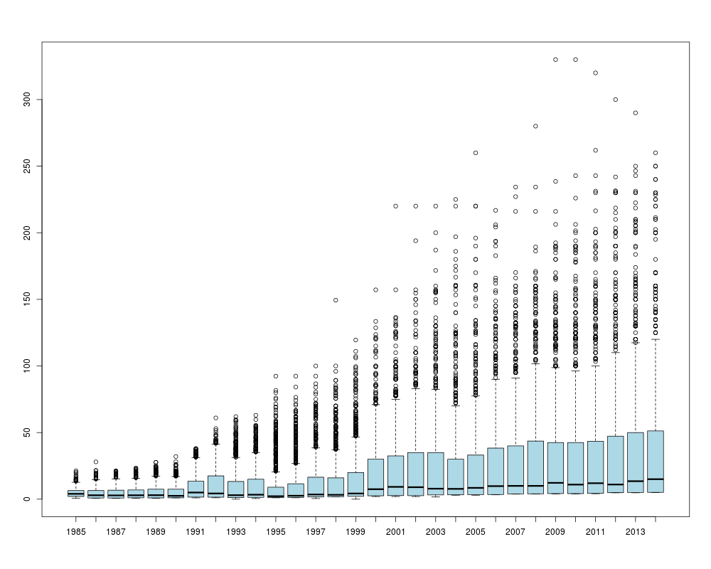
# see the whole distribution
boxplot(salary/100000 ~ yearID, data=Salaries, col="lightblue")

# add salary to Batting data
batting <- merge(Batting, 
                 Salaries[,c("playerID", "yearID", "teamID", "salary")], 
                 by=c("playerID", "yearID", "teamID"), all.x=TRUE)
str(batting)

#######################################
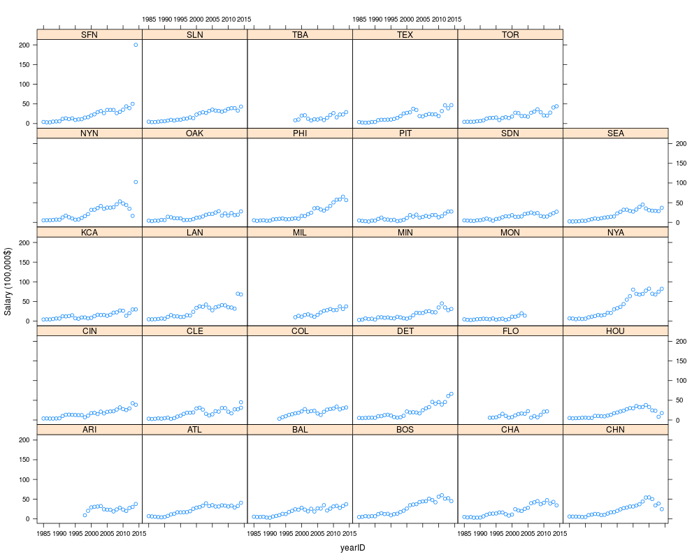
# Average salaries by teams, over years
#######################################

require(plyr)
avesal <- ddply(Salaries, .(yearID, teamID, lgID), summarise, 
	salary= mean(salary)/100000)

# remove infrequent teams
tcount <- table(avesal$teamID)
avesal <- subset(avesal, avesal$teamID %in% names(tcount)[tcount>=15], drop=TRUE)
avesal$teamID <- factor(avesal$teamID, levels=names(tcount)[tcount>=15])

require(lattice)
xyplot(salary ~ yearID | teamID, data=avesal, ylab="Salary (100,000$)")

Results

R version 3.3.1 (2016-06-21) -- "Bug in Your Hair"
Copyright (C) 2016 The R Foundation for Statistical Computing
Platform: x86_64-pc-linux-gnu (64-bit)

R is free software and comes with ABSOLUTELY NO WARRANTY.
You are welcome to redistribute it under certain conditions.
Type 'license()' or 'licence()' for distribution details.

R is a collaborative project with many contributors.
Type 'contributors()' for more information and
'citation()' on how to cite R or R packages in publications.

Type 'demo()' for some demos, 'help()' for on-line help, or
'help.start()' for an HTML browser interface to help.
Type 'q()' to quit R.

> library(Lahman)
> png(filename="/home/ddbj/snapshot/RGM3/R_CC/result/Lahman/Salaries.Rd_%03d_medium.png", width=480, height=480)
> ### Name: Salaries
> ### Title: Salaries table
> ### Aliases: Salaries
> ### Keywords: datasets
> 
> ### ** Examples
> 
> # what years are included?
> summary(Salaries$yearID)
   Min. 1st Qu.  Median    Mean 3rd Qu.    Max. 
   1985    1993    2000    2000    2007    2014 
> # how many players included each year?
> table(Salaries$yearID)

1985 1986 1987 1988 1989 1990 1991 1992 1993 1994 1995 1996 1997 1998 1999 2000 
 550  738  627  663  711  867  685  769  923  884  986  931  925  998 1006  836 
2001 2002 2003 2004 2005 2006 2007 2008 2009 2010 2011 2012 2013 2014 
 860  846  827  831  831  819  842  856  813  830  839  848  815  802 
> 
> # Team salary data
> 
> require(plyr)
Loading required package: plyr
> 
> # Total team salaries by league, team and year
> teamSalaries <- ddply(Salaries, .(lgID, teamID, yearID), summarise,
+                        Salary = sum(as.numeric(salary)))
> 
> # Arrange in decreasing order within year and league:
> teamSalaries <- ddply(teamSalaries, .(yearID, lgID), arrange, desc(Salary))
> 
> #######################################
> # Highest paid players each year:
> maxSal <- ddply(Salaries, .(yearID), subset, salary == max(salary))
> names <- apply(t(sapply(maxSal$playerID, playerInfo))[,2:3], 2, paste)
> maxSal <- cbind(maxSal, names)
> maxSal
   yearID teamID lgID  playerID   salary nameFirst   nameLast
1    1985    PHI   NL schmimi01  2130300      Mike    Schmidt
2    1986    NYN   NL fostege01  2800000    George     Foster
3    1987    PHI   NL schmimi01  2127333      Mike    Schmidt
4    1988    SLN   NL smithoz01  2340000     Ozzie      Smith
5    1989    LAN   NL hershor01  2766667      Orel  Hershiser
6    1990    ML4   AL yountro01  3200000     Robin      Yount
7    1991    LAN   NL strawda01  3800000    Darryl Strawberry
8    1992    NYN   NL bonilbo01  6100000     Bobby    Bonilla
9    1993    NYN   NL bonilbo01  6200000     Bobby    Bonilla
10   1994    NYN   NL bonilbo01  6300000     Bobby    Bonilla
11   1995    DET   AL fieldce01  9237500     Cecil    Fielder
12   1996    DET   AL fieldce01  9237500     Cecil    Fielder
13   1997    CHA   AL belleal01 10000000    Albert      Belle
14   1998    FLO   NL sheffga01 14936667      Gary  Sheffield
15   1999    BAL   AL belleal01 11949794    Albert      Belle
16   2000    LAN   NL brownke01 15714286     Kevin      Brown
17   2001    TEX   AL rodrial01 22000000      Alex  Rodriguez
18   2002    TEX   AL rodrial01 22000000      Alex  Rodriguez
19   2003    TEX   AL rodrial01 22000000      Alex  Rodriguez
20   2004    BOS   AL ramirma02 22500000     Manny    Ramirez
21   2005    NYA   AL rodrial01 26000000      Alex  Rodriguez
22   2006    NYA   AL rodrial01 21680727      Alex  Rodriguez
23   2007    NYA   AL giambja01 23428571     Jason     Giambi
24   2008    NYA   AL rodrial01 28000000      Alex  Rodriguez
25   2009    NYA   AL rodrial01 33000000      Alex  Rodriguez
26   2010    NYA   AL rodrial01 33000000      Alex  Rodriguez
27   2011    NYA   AL rodrial01 32000000      Alex  Rodriguez
28   2012    NYA   AL rodrial01 30000000      Alex  Rodriguez
29   2013    NYA   AL rodrial01 29000000      Alex  Rodriguez
30   2014    LAN   NL greinza01 26000000      Zack    Greinke
> plot(salary/100000 ~ yearID, data=maxSal, type='b', ylab='Salary (100,000$)')
> # see the whole distribution
> boxplot(salary/100000 ~ yearID, data=Salaries, col="lightblue")
> 
> # add salary to Batting data
> batting <- merge(Batting, 
+                  Salaries[,c("playerID", "yearID", "teamID", "salary")], 
+                  by=c("playerID", "yearID", "teamID"), all.x=TRUE)
> str(batting)
'data.frame':	99846 obs. of  23 variables:
 $ playerID: chr  "aardsda01" "aardsda01" "aardsda01" "aardsda01" ...
 $ yearID  : int  2004 2006 2007 2008 2009 2010 2012 2013 1954 1955 ...
 $ teamID  : Factor w/ 149 levels "ALT","ANA","ARI",..: 117 35 33 16 116 116 93 94 80 80 ...
 $ stint   : int  1 1 1 1 1 1 1 1 1 1 ...
 $ lgID    : Factor w/ 7 levels "AA","AL","FL",..: 5 5 2 2 2 2 2 5 5 5 ...
 $ G       : int  11 45 25 47 73 53 1 43 122 153 ...
 $ AB      : int  0 2 0 1 0 0 0 0 468 602 ...
 $ R       : int  0 0 0 0 0 0 0 0 58 105 ...
 $ H       : int  0 0 0 0 0 0 0 0 131 189 ...
 $ X2B     : int  0 0 0 0 0 0 0 0 27 37 ...
 $ X3B     : int  0 0 0 0 0 0 0 0 6 9 ...
 $ HR      : int  0 0 0 0 0 0 0 0 13 27 ...
 $ RBI     : int  0 0 0 0 0 0 0 0 69 106 ...
 $ SB      : int  0 0 0 0 0 0 0 0 2 3 ...
 $ CS      : int  0 0 0 0 0 0 0 0 2 1 ...
 $ BB      : int  0 0 0 0 0 0 0 0 28 49 ...
 $ SO      : int  0 0 0 1 0 0 0 0 39 61 ...
 $ IBB     : int  0 0 0 0 0 0 0 0 NA 5 ...
 $ HBP     : int  0 0 0 0 0 0 0 0 3 3 ...
 $ SH      : int  0 1 0 0 0 0 0 0 6 7 ...
 $ SF      : int  0 0 0 0 0 0 0 0 4 4 ...
 $ GIDP    : int  0 0 0 0 0 0 0 0 13 20 ...
 $ salary  : int  300000 NA 387500 403250 419000 2750000 500000 NA NA NA ...
> 
> #######################################
> # Average salaries by teams, over years
> #######################################
> 
> require(plyr)
> avesal <- ddply(Salaries, .(yearID, teamID, lgID), summarise, 
+ 	salary= mean(salary)/100000)
> 
> # remove infrequent teams
> tcount <- table(avesal$teamID)
> avesal <- subset(avesal, avesal$teamID %in% names(tcount)[tcount>=15], drop=TRUE)
> avesal$teamID <- factor(avesal$teamID, levels=names(tcount)[tcount>=15])
> 
> require(lattice)
Loading required package: lattice
> xyplot(salary ~ yearID | teamID, data=avesal, ylab="Salary (100,000$)")
> 
> 
> 
> 
> 
> 
> dev.off()
null device 
          1 
>