Supported by Dr. Osamu Ogasawara and  . . |
|
Last data update: 2014.03.03 |
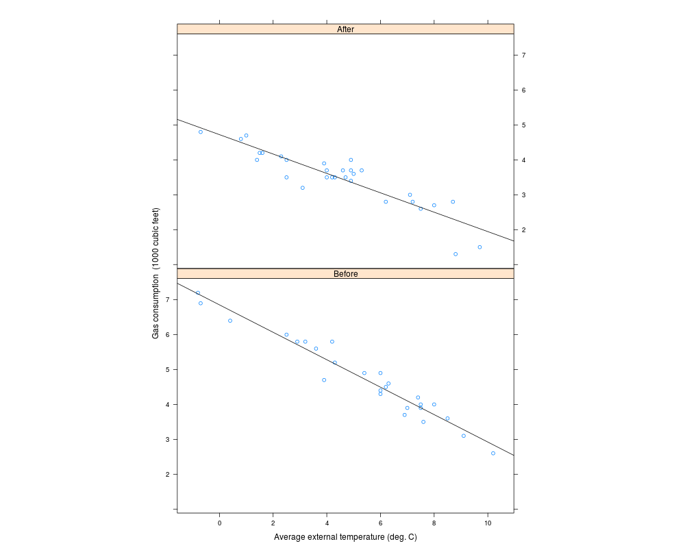
House Insulation: Whiteside's DataDescriptionMr Derek Whiteside of the UK Building Research Station recorded the weekly gas consumption and average external temperature at his own house in south-east England for two heating seasons, one of 26 weeks before, and one of 30 weeks after cavity-wall insulation was installed. The object of the exercise was to assess the effect of the insulation on gas consumption. Usagewhiteside FormatThe
SourceA data set collected in the 1960s by Mr Derek Whiteside of the UK Building Research Station. Reported by Hand, D. J., Daly, F., McConway, K., Lunn, D. and Ostrowski, E. eds (1993) A Handbook of Small Data Sets. Chapman & Hall, p. 69. ReferencesVenables, W. N. and Ripley, B. D. (2002) Modern Applied Statistics with S. Fourth edition. Springer. Examples
require(lattice)
xyplot(Gas ~ Temp | Insul, whiteside, panel =
  function(x, y, ...) {
    panel.xyplot(x, y, ...)
    panel.lmline(x, y, ...)
  }, xlab = "Average external temperature (deg. C)",
  ylab = "Gas consumption  (1000 cubic feet)", aspect = "xy",
  strip = function(...) strip.default(..., style = 1))

gasB <- lm(Gas ~ Temp, whiteside, subset = Insul=="Before")
gasA <- update(gasB, subset = Insul=="After")
summary(gasB)
summary(gasA)
gasBA <- lm(Gas ~ Insul/Temp - 1, whiteside)
summary(gasBA)

gasQ <- lm(Gas ~ Insul/(Temp + I(Temp^2)) - 1, whiteside)
coef(summary(gasQ))

gasPR <- lm(Gas ~ Insul + Temp, whiteside)
anova(gasPR, gasBA)
options(contrasts = c("contr.treatment", "contr.poly"))
gasBA1 <- lm(Gas ~ Insul*Temp, whiteside)
coef(summary(gasBA1))
Results
R version 3.3.1 (2016-06-21) -- "Bug in Your Hair"
Copyright (C) 2016 The R Foundation for Statistical Computing
Platform: x86_64-pc-linux-gnu (64-bit)

R is free software and comes with ABSOLUTELY NO WARRANTY.
You are welcome to redistribute it under certain conditions.
Type 'license()' or 'licence()' for distribution details.

R is a collaborative project with many contributors.
Type 'contributors()' for more information and
'citation()' on how to cite R or R packages in publications.

Type 'demo()' for some demos, 'help()' for on-line help, or
'help.start()' for an HTML browser interface to help.
Type 'q()' to quit R.

> library(MASS)
> png(filename="/home/ddbj/snapshot/RGM3/R_CC/result/MASS/whiteside.Rd_%03d_medium.png", width=480, height=480)
> ### Name: whiteside
> ### Title: House Insulation: Whiteside's Data
> ### Aliases: whiteside
> ### Keywords: datasets
>
> ### ** Examples
>
> require(lattice)
Loading required package: lattice
> xyplot(Gas ~ Temp | Insul, whiteside, panel =
+   function(x, y, ...) {
+     panel.xyplot(x, y, ...)
+     panel.lmline(x, y, ...)
+   }, xlab = "Average external temperature (deg. C)",
+   ylab = "Gas consumption  (1000 cubic feet)", aspect = "xy",
+   strip = function(...) strip.default(..., style = 1))
>
> gasB <- lm(Gas ~ Temp, whiteside, subset = Insul=="Before")
> gasA <- update(gasB, subset = Insul=="After")
> summary(gasB)

Call:
lm(formula = Gas ~ Temp, data = whiteside, subset = Insul ==
    "Before")

Residuals:
     Min       1Q   Median       3Q      Max
-0.62020 -0.19947  0.06068  0.16770  0.59778

Coefficients:
            Estimate Std. Error t value Pr(>|t|)
(Intercept)  6.85383    0.11842   57.88   <2e-16 ***
Temp        -0.39324    0.01959  -20.08   <2e-16 ***
---
Signif. codes:  0 '***' 0.001 '**' 0.01 '*' 0.05 '.' 0.1 ' ' 1

Residual standard error: 0.2813 on 24 degrees of freedom
Multiple R-squared:  0.9438,	Adjusted R-squared:  0.9415
F-statistic: 403.1 on 1 and 24 DF,  p-value: < 2.2e-16

> summary(gasA)

Call:
lm(formula = Gas ~ Temp, data = whiteside, subset = Insul ==
    "After")

Residuals:
     Min       1Q   Median       3Q      Max
-0.97802 -0.11082  0.02672  0.25294  0.63803

Coefficients:
            Estimate Std. Error t value Pr(>|t|)
(Intercept)  4.72385    0.12974   36.41  < 2e-16 ***
Temp        -0.27793    0.02518  -11.04 1.05e-11 ***
---
Signif. codes:  0 '***' 0.001 '**' 0.01 '*' 0.05 '.' 0.1 ' ' 1

Residual standard error: 0.3548 on 28 degrees of freedom
Multiple R-squared:  0.8131,	Adjusted R-squared:  0.8064
F-statistic: 121.8 on 1 and 28 DF,  p-value: 1.046e-11

> gasBA <- lm(Gas ~ Insul/Temp - 1, whiteside)
> summary(gasBA)

Call:
lm(formula = Gas ~ Insul/Temp - 1, data = whiteside)

Residuals:
     Min       1Q   Median       3Q      Max
-0.97802 -0.18011  0.03757  0.20930  0.63803

Coefficients:
                 Estimate Std. Error t value Pr(>|t|)
InsulBefore       6.85383    0.13596   50.41   <2e-16 ***
InsulAfter        4.72385    0.11810   40.00   <2e-16 ***
InsulBefore:Temp -0.39324    0.02249  -17.49   <2e-16 ***
InsulAfter:Temp  -0.27793    0.02292  -12.12   <2e-16 ***
---
Signif. codes:  0 '***' 0.001 '**' 0.01 '*' 0.05 '.' 0.1 ' ' 1

Residual standard error: 0.323 on 52 degrees of freedom
Multiple R-squared:  0.9946,	Adjusted R-squared:  0.9942
F-statistic:  2391 on 4 and 52 DF,  p-value: < 2.2e-16

>
> gasQ <- lm(Gas ~ Insul/(Temp + I(Temp^2)) - 1, whiteside)
> coef(summary(gasQ))
                          Estimate  Std. Error   t value     Pr(>|t|)
InsulBefore            6.759215179 0.150786777 44.826312 4.854615e-42
InsulAfter             4.496373920 0.160667904 27.985514 3.302572e-32
InsulBefore:Temp      -0.317658735 0.062965170 -5.044991 6.362323e-06
InsulAfter:Temp       -0.137901603 0.073058019 -1.887563 6.489554e-02
InsulBefore:I(Temp^2) -0.008472572 0.006624737 -1.278930 2.068259e-01
InsulAfter:I(Temp^2)  -0.014979455 0.007447107 -2.011446 4.968398e-02
>
> gasPR <- lm(Gas ~ Insul + Temp, whiteside)
> anova(gasPR, gasBA)
Analysis of Variance Table

Model 1: Gas ~ Insul + Temp
Model 2: Gas ~ Insul/Temp - 1
  Res.Df    RSS Df Sum of Sq      F    Pr(>F)
1     53 6.7704
2     52 5.4252  1    1.3451 12.893 0.0007307 ***
---
Signif. codes:  0 '***' 0.001 '**' 0.01 '*' 0.05 '.' 0.1 ' ' 1
> options(contrasts = c("contr.treatment", "contr.poly"))
> gasBA1 <- lm(Gas ~ Insul*Temp, whiteside)
> coef(summary(gasBA1))
                  Estimate Std. Error    t value     Pr(>|t|)
(Intercept)      6.8538277 0.13596397  50.409146 7.997414e-46
InsulAfter      -2.1299780 0.18009172 -11.827185 2.315921e-16
Temp            -0.3932388 0.02248703 -17.487358 1.976009e-23
InsulAfter:Temp  0.1153039 0.03211212   3.590665 7.306852e-04
>
>
>
>
>
> dev.off()
null device
          1
>
|