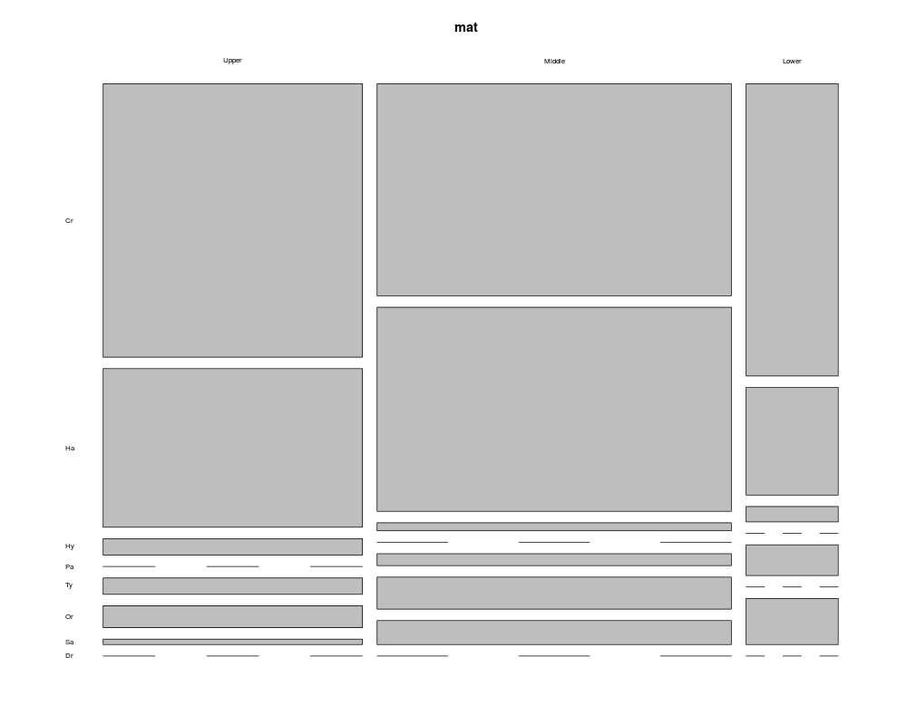
Hell Creek Dinosaur Data

Description

Counts of dinosaur families found in three stratigraphic levels of the Cretaceous period in the Hell Creek formation in North Dakota. The eight families are the Ceratopsidae (Ce), Hadrosauridae (Ha), Hypsilophodontidae (Hy), Pachycephalosauridae (Pa), Tyrannosauridae (Ty), Ornithomimidae (Or), Sauronithoididae (Sa) and Dromiaeosauridae (Dr).

Usage

data(HCD)

Format

A data frame with 3 observations on the following 9 variables.

Level

a factor with levels Lower, Middle, Upper, specifiyng the stratigraphic levels

Cr

a numeric vector, counts of the Ceratopsidae

Ha

a numeric vector, counts of the Hadrosauridae

Hy

a numeric vector, counts of the Hypsilophodontidae

Pa

a numeric vector, counts of the Pachycephalosauridae

Ty

a numeric vector, counts of the Tyrannosauridae

Or

a numeric vector, counts of the Ornithomimidae

Sa

a numeric vector, counts of the Sauronithoididae

Dr

a numeric vector, counts of the Dromiaeosauridae

Source

Table 1 in: Rogers, JA and Hsu, JC (2001): Multiple Comparisons of Biodiversity. Biometrical Journal 43, 617-625.

References

Sheehan, P.M., et al. (1991): Sudden extinction of the Dinosaurs: Latest Cretaceous, Upper Great Plains, U.S.A. Science 254, 835-839.

Examples

data(HCD)
str(HCD)
HCD

mat<-as.matrix(HCD[,-c(1)])

rownames(mat)<-HCD$Level

mosaicplot(mat, las=1)

estSimpsonf(X=HCD[,-c(1)], f=HCD$Level)

estShannonf(X=HCD[,-c(1)], f=HCD$Level)

Results

R version 3.3.1 (2016-06-21) -- "Bug in Your Hair"
Copyright (C) 2016 The R Foundation for Statistical Computing
Platform: x86_64-pc-linux-gnu (64-bit)

R is free software and comes with ABSOLUTELY NO WARRANTY.
You are welcome to redistribute it under certain conditions.
Type 'license()' or 'licence()' for distribution details.

R is a collaborative project with many contributors.
Type 'contributors()' for more information and
'citation()' on how to cite R or R packages in publications.

Type 'demo()' for some demos, 'help()' for on-line help, or
'help.start()' for an HTML browser interface to help.
Type 'q()' to quit R.

> library(MCPAN)
> png(filename="/home/ddbj/snapshot/RGM3/R_CC/result/MCPAN/HCD.Rd_%03d_medium.png", width=480, height=480)
> ### Name: HCD
> ### Title: Hell Creek Dinosaur Data
> ### Aliases: HCD
> ### Keywords: datasets
> 
> ### ** Examples
> 
> 
> data(HCD)
> str(HCD)
'data.frame':	3 obs. of  9 variables:
 $ Level: Factor w/ 3 levels "Lower","Middle",..: 3 2 1
 $ Cr   : int  50 53 19
 $ Ha   : int  29 51 7
 $ Hy   : int  3 2 1
 $ Pa   : int  0 0 0
 $ Ty   : int  3 3 2
 $ Or   : int  4 8 0
 $ Sa   : int  1 6 3
 $ Dr   : int  0 0 0
> HCD
   Level Cr Ha Hy Pa Ty Or Sa Dr
1  Upper 50 29  3  0  3  4  1  0
2 Middle 53 51  2  0  3  8  6  0
3  Lower 19  7  1  0  2  0  3  0
> 
> mat<-as.matrix(HCD[,-c(1)])
> 
> rownames(mat)<-HCD$Level
> 
> mosaicplot(mat, las=1)
> 
> estSimpsonf(X=HCD[,-c(1)], f=HCD$Level)
$estimate
    Lower    Middle     Upper 
0.6048387 0.6401439 0.5897628 

$varest
       Lower       Middle        Upper 
0.0064696035 0.0006253136 0.0014393560 

$table
       Cr Ha Hy Pa Ty Or Sa Dr
Lower  19  7  1  0  2  0  3  0
Middle 53 51  2  0  3  8  6  0
Upper  50 29  3  0  3  4  1  0

> 
> estShannonf(X=HCD[,-c(1)], f=HCD$Level)
$estimate
   Lower   Middle    Upper 
1.254866 1.238877 1.145481 

$estraw
   Lower   Middle    Upper 
1.145491 1.210422 1.106592 

$estHBCo0
   Lower   Middle    Upper 
1.207991 1.230747 1.134370 

$varest
      Lower      Middle       Upper 
0.022987521 0.005728593 0.008974520 

$table
       Cr Ha Hy Pa Ty Or Sa Dr
Lower  19  7  1  0  2  0  3  0
Middle 53 51  2  0  3  8  6  0
Upper  50 29  3  0  3  4  1  0

> 
> 
> 
> 
> 
> 
> dev.off()
null device 
          1 
>