Artificially generated data alike that of Suspension bead arrays

Description

The data that has similarity to Suspension bead arrays data.

Usage

data(sba)

Format

A list that consists of "plate" which is a factor of plate number, "X" that contains measured values where columns are targets and rows are samples (or observations).

Examples

data(sba)

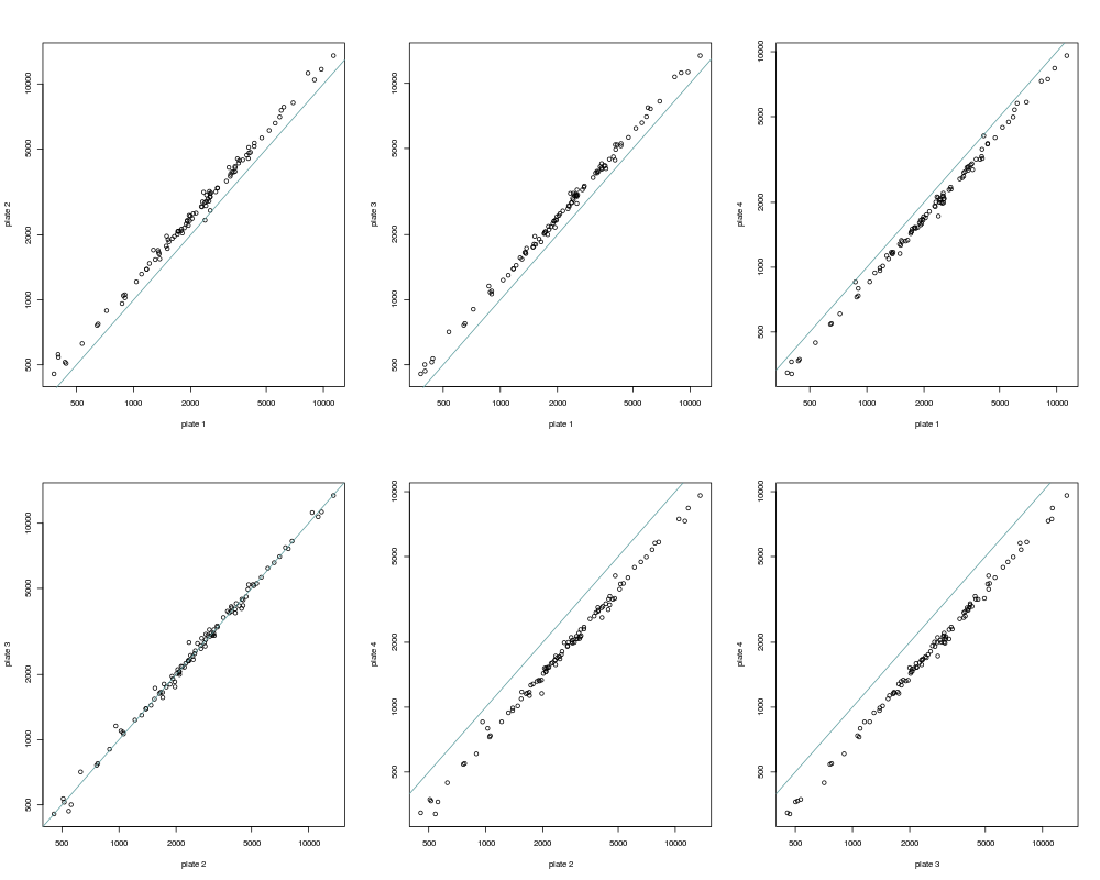
# plot to check difference of geometric mean of every target between plates
sba_gm <- by(sba$X, sba$plate, apply, 2, function(x) exp(mean(log(x))))	
par(mfrow= c(2, 3))
apply(combn(4, 2), 2, function(ea) {
	plot(sba_gm[[ea[1]]], sba_gm[[ea[2]]], xlab= names(sba_gm)[ea[1]], 
	     ylab= names(sba_gm)[ea[2]], log= "xy", asp= 1)
	abline(0, 1, col= "cadetblue")
})

# show first 10 observations in plate 1 and plate 2
print(sba$X[c(1:10, 97:106), 1:10])		

Results

R version 3.3.1 (2016-06-21) -- "Bug in Your Hair"
Copyright (C) 2016 The R Foundation for Statistical Computing
Platform: x86_64-pc-linux-gnu (64-bit)

R is free software and comes with ABSOLUTELY NO WARRANTY.
You are welcome to redistribute it under certain conditions.
Type 'license()' or 'licence()' for distribution details.

R is a collaborative project with many contributors.
Type 'contributors()' for more information and
'citation()' on how to cite R or R packages in publications.

Type 'demo()' for some demos, 'help()' for on-line help, or
'help.start()' for an HTML browser interface to help.
Type 'q()' to quit R.

> library(MDimNormn)
> png(filename="/home/ddbj/snapshot/RGM3/R_CC/result/MDimNormn/sba.Rd_%03d_medium.png", width=480, height=480)
> ### Name: SBA
> ### Title: Artificially generated data alike that of Suspension bead arrays
> ### Aliases: sba
> ### Keywords: datasets
> 
> ### ** Examples
> 
> data(sba)
> 
> # plot to check difference of geometric mean of every target between plates
> sba_gm <- by(sba$X, sba$plate, apply, 2, function(x) exp(mean(log(x))))	
> par(mfrow= c(2, 3))
> apply(combn(4, 2), 2, function(ea) {
+ 	plot(sba_gm[[ea[1]]], sba_gm[[ea[2]]], xlab= names(sba_gm)[ea[1]], 
+ 	     ylab= names(sba_gm)[ea[2]], log= "xy", asp= 1)
+ 	abline(0, 1, col= "cadetblue")
+ })
NULL
> 
> # show first 10 observations in plate 1 and plate 2
> print(sba$X[c(1:10, 97:106), 1:10])		
       T1    T2   T3   T4   T5   T6   T7   T8   T9  T10
S1   1940  4946 1342 1122 1332 3066 1610 2094 2822 4763
S2   2735  6688 1978 1534 1839 4575 2225 3066 3915 6386
S3   2338  5990 1593 1279 1594 3748 1869 2332 3338 5493
S4   2573  6070 1816 1390 1683 3735 1917 2551 3624 5757
S5   1841  4953 1262 1035 1283 2867 1586 1992 2675 4229
S6   2086  4816 1401 1105 1297 3132 1572 2174 2836 4534
S7   1883  4493 1313 1007 1294 2965 1449 2028 2663 4154
S8   2342  6495 1778 1368 1839 3860 2095 2692 3653 5493
S9   2866  6669 1906 1499 1899 4363 2045 2764 3936 6245
S10  2862  7927 2071 1649 1898 4662 2429 3019 4249 6874
S97  2296  6219 1513 1283 1611 3591 1880 2383 3293 5129
S98  2567  6783 1784 1492 1751 4135 2155 2785 3834 5722
S99  3619 10284 2583 2185 2477 6090 3144 3872 5248 8282
S100 1748  4954 1306 1129 1307 3126 1567 2269 2782 4684
S101 2164  6116 1551 1398 1530 3853 1777 2452 3267 5229
S102 2424  6051 1571 1340 1668 3846 1978 2628 3372 5161
S103 3302  9345 2345 1949 2194 5443 2890 3771 4855 7808
S104 2443  7092 1807 1442 1673 3987 2113 2603 3518 5896
S105 2654  7335 1937 1672 1894 4499 2136 2873 4103 6229
S106 3072  8237 2053 1823 2095 4910 2533 3186 4798 7016
> 
> 
> 
> 
> 
> 
> dev.off()
null device 
          1 
>