Flow of the River Nile

Description

Measurements of the annual flow of the river Nile at Aswan (formerly Assuan), 1871–1970, in 10^8 m^3, “with apparent changepoint near 1898” (Cobb(1978), Table 1, p.249).

Usage

Nile

Format

A time series of length 100.

Source

Durbin, J. and Koopman, S. J. (2001) Time Series Analysis by State Space Methods. Oxford University Press. http://www.ssfpack.com/DKbook.html

References

Balke, N. S. (1993) Detecting level shifts in time series. Journal of Business and Economic Statistics 11, 81–92.

Cobb, G. W. (1978) The problem of the Nile: conditional solution to a change-point problem. Biometrika 65, 243–51.

Examples

require(stats); require(graphics)
par(mfrow = c(2, 2))
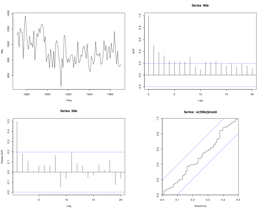
plot(Nile)
acf(Nile)
pacf(Nile)
ar(Nile) # selects order 2
cpgram(ar(Nile)$resid)
par(mfrow = c(1, 1))
arima(Nile, c(2, 0, 0))

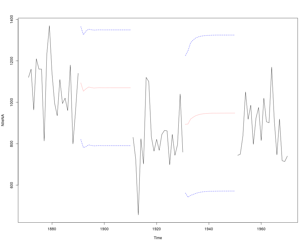
## Now consider missing values, following Durbin & Koopman
NileNA <- Nile
NileNA[c(21:40, 61:80)] <- NA
arima(NileNA, c(2, 0, 0))
plot(NileNA)
pred <-
   predict(arima(window(NileNA, 1871, 1890), c(2, 0, 0)), n.ahead = 20)
lines(pred$pred, lty = 3, col = "red")
lines(pred$pred + 2*pred$se, lty = 2, col = "blue")
lines(pred$pred - 2*pred$se, lty = 2, col = "blue")
pred <-
   predict(arima(window(NileNA, 1871, 1930), c(2, 0, 0)), n.ahead = 20)
lines(pred$pred, lty = 3, col = "red")
lines(pred$pred + 2*pred$se, lty = 2, col = "blue")
lines(pred$pred - 2*pred$se, lty = 2, col = "blue")

## Structural time series models
par(mfrow = c(3, 1))
plot(Nile)
## local level model
(fit <- StructTS(Nile, type = "level"))
lines(fitted(fit), lty = 2)              # contemporaneous smoothing
lines(tsSmooth(fit), lty = 2, col = 4)   # fixed-interval smoothing
plot(residuals(fit)); abline(h = 0, lty = 3)
## local trend model
(fit2 <- StructTS(Nile, type = "trend")) ## constant trend fitted
pred <- predict(fit, n.ahead = 30)
## with 50% confidence interval
ts.plot(Nile, pred$pred,
        pred$pred + 0.67*pred$se, pred$pred -0.67*pred$se)

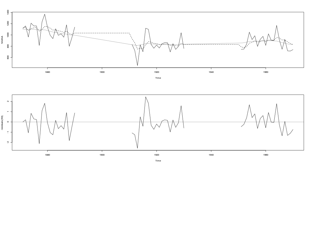
## Now consider missing values
plot(NileNA)
(fit3 <- StructTS(NileNA, type = "level"))
lines(fitted(fit3), lty = 2)
lines(tsSmooth(fit3), lty = 3)
plot(residuals(fit3)); abline(h = 0, lty = 3)

Results

R version 3.3.1 (2016-06-21) -- "Bug in Your Hair"
Copyright (C) 2016 The R Foundation for Statistical Computing
Platform: x86_64-pc-linux-gnu (64-bit)

R is free software and comes with ABSOLUTELY NO WARRANTY.
You are welcome to redistribute it under certain conditions.
Type 'license()' or 'licence()' for distribution details.

R is a collaborative project with many contributors.
Type 'contributors()' for more information and
'citation()' on how to cite R or R packages in publications.

Type 'demo()' for some demos, 'help()' for on-line help, or
'help.start()' for an HTML browser interface to help.
Type 'q()' to quit R.

> library(datasets)
> png(filename="/home/ddbj/snapshot/RGM3/R_rel/result/datasets/Nile.Rd_%03d_medium.png", width=480, height=480)
> ### Name: Nile
> ### Title: Flow of the River Nile
> ### Aliases: Nile
> ### Keywords: datasets
> 
> ### ** Examples
> 
> require(stats); require(graphics)
> par(mfrow = c(2, 2))
> plot(Nile)
> acf(Nile)
> pacf(Nile)
> ar(Nile) # selects order 2

Call:
ar(x = Nile)

Coefficients:
     1       2  
0.4081  0.1812  

Order selected 2  sigma^2 estimated as  21247
> cpgram(ar(Nile)$resid)
> par(mfrow = c(1, 1))
> arima(Nile, c(2, 0, 0))

Call:
arima(x = Nile, order = c(2, 0, 0))

Coefficients:
         ar1     ar2  intercept
      0.4096  0.1987   919.8397
s.e.  0.0974  0.0990    35.6410

sigma^2 estimated as 20291:  log likelihood = -637.98,  aic = 1283.96
> 
> ## Now consider missing values, following Durbin & Koopman
> NileNA <- Nile
> NileNA[c(21:40, 61:80)] <- NA
> arima(NileNA, c(2, 0, 0))

Call:
arima(x = NileNA, order = c(2, 0, 0))

Coefficients:
         ar1     ar2  intercept
      0.3622  0.1678   918.3103
s.e.  0.1273  0.1323    39.5037

sigma^2 estimated as 23676:  log likelihood = -387.7,  aic = 783.41
> plot(NileNA)
> pred <-
+    predict(arima(window(NileNA, 1871, 1890), c(2, 0, 0)), n.ahead = 20)
> lines(pred$pred, lty = 3, col = "red")
> lines(pred$pred + 2*pred$se, lty = 2, col = "blue")
> lines(pred$pred - 2*pred$se, lty = 2, col = "blue")
> pred <-
+    predict(arima(window(NileNA, 1871, 1930), c(2, 0, 0)), n.ahead = 20)
> lines(pred$pred, lty = 3, col = "red")
> lines(pred$pred + 2*pred$se, lty = 2, col = "blue")
> lines(pred$pred - 2*pred$se, lty = 2, col = "blue")
> 
> ## Structural time series models
> par(mfrow = c(3, 1))
> plot(Nile)
> ## local level model
> (fit <- StructTS(Nile, type = "level"))

Call:
StructTS(x = Nile, type = "level")

Variances:
  level  epsilon  
   1469    15099  
> lines(fitted(fit), lty = 2)              # contemporaneous smoothing
> lines(tsSmooth(fit), lty = 2, col = 4)   # fixed-interval smoothing
> plot(residuals(fit)); abline(h = 0, lty = 3)
> ## local trend model
> (fit2 <- StructTS(Nile, type = "trend")) ## constant trend fitted

Call:
StructTS(x = Nile, type = "trend")

Variances:
  level    slope  epsilon  
   1427        0    15047  
> pred <- predict(fit, n.ahead = 30)
> ## with 50% confidence interval
> ts.plot(Nile, pred$pred,
+         pred$pred + 0.67*pred$se, pred$pred -0.67*pred$se)
> 
> ## Now consider missing values
> plot(NileNA)
> (fit3 <- StructTS(NileNA, type = "level"))

Call:
StructTS(x = NileNA, type = "level")

Variances:
  level  epsilon  
  685.8  17899.8  
> lines(fitted(fit3), lty = 2)
> lines(tsSmooth(fit3), lty = 3)
> plot(residuals(fit3)); abline(h = 0, lty = 3)
> 
> 
> 
> 
> 
> dev.off()
null device 
          1 
>