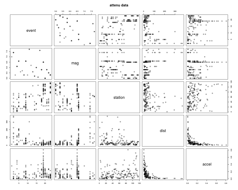
The Joyner–Boore Attenuation Data

Description

This data gives peak accelerations measured at various observation stations for 23 earthquakes in California. The data have been used by various workers to estimate the attenuating affect of distance on ground acceleration.

Usage

attenu

Format

A data frame with 182 observations on 5 variables.

Source

Joyner, W.B., D.M. Boore and R.D. Porcella (1981). Peak horizontal acceleration and velocity from strong-motion records including records from the 1979 Imperial Valley, California earthquake. USGS Open File report 81-365. Menlo Park, Ca.

References

Boore, D. M. and Joyner, W.B.(1982) The empirical prediction of ground motion, Bull. Seism. Soc. Am., 72, S269–S268.

Bolt, B. A. and Abrahamson, N. A. (1982) New attenuation relations for peak and expected accelerations of strong ground motion, Bull. Seism. Soc. Am., 72, 2307–2321.

Bolt B. A. and Abrahamson, N. A. (1983) Reply to W. B. Joyner & D. M. Boore's “Comments on: New attenuation relations for peak and expected accelerations for peak and expected accelerations of strong ground motion”, Bull. Seism. Soc. Am., 73, 1481–1483.

Brillinger, D. R. and Preisler, H. K. (1984) An exploratory analysis of the Joyner-Boore attenuation data, Bull. Seism. Soc. Am., 74, 1441–1449.

Brillinger, D. R. and Preisler, H. K. (1984) Further analysis of the Joyner-Boore attenuation data. Manuscript.

Examples

require(graphics)
## check the data class of the variables
sapply(attenu, data.class)
summary(attenu)
pairs(attenu, main = "attenu data")
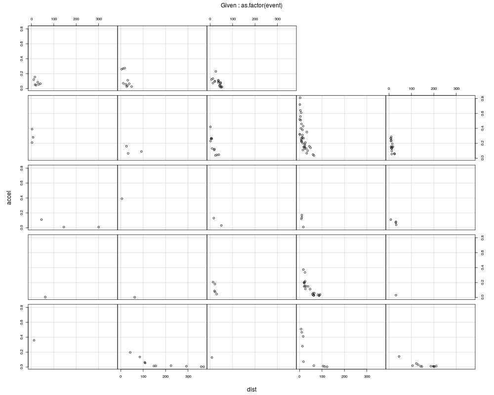
coplot(accel ~ dist | as.factor(event), data = attenu, show.given = FALSE)
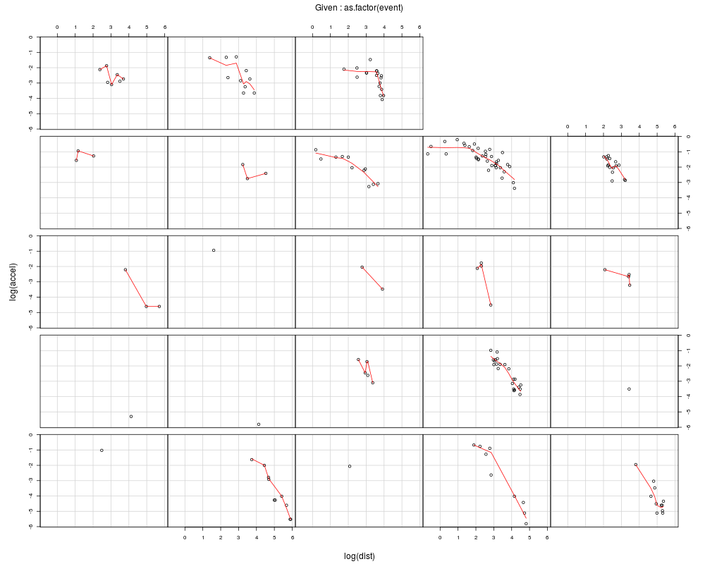
coplot(log(accel) ~ log(dist) | as.factor(event),
       data = attenu, panel = panel.smooth, show.given = FALSE)

Results

R version 3.3.1 (2016-06-21) -- "Bug in Your Hair"
Copyright (C) 2016 The R Foundation for Statistical Computing
Platform: x86_64-pc-linux-gnu (64-bit)

R is free software and comes with ABSOLUTELY NO WARRANTY.
You are welcome to redistribute it under certain conditions.
Type 'license()' or 'licence()' for distribution details.

R is a collaborative project with many contributors.
Type 'contributors()' for more information and
'citation()' on how to cite R or R packages in publications.

Type 'demo()' for some demos, 'help()' for on-line help, or
'help.start()' for an HTML browser interface to help.
Type 'q()' to quit R.

> library(datasets)
> png(filename="/home/ddbj/snapshot/RGM3/R_rel/result/datasets/attenu.Rd_%03d_medium.png", width=480, height=480)
> ### Name: attenu
> ### Title: The Joyner-Boore Attenuation Data
> ### Aliases: attenu
> ### Keywords: datasets
> 
> ### ** Examples
> 
> require(graphics)
> ## check the data class of the variables
> sapply(attenu, data.class)
    event       mag   station      dist     accel 
"numeric" "numeric"  "factor" "numeric" "numeric" 
> summary(attenu)
     event            mag           station         dist       
 Min.   : 1.00   Min.   :5.000   117    :  5   Min.   :  0.50  
 1st Qu.: 9.00   1st Qu.:5.300   1028   :  4   1st Qu.: 11.32  
 Median :18.00   Median :6.100   113    :  4   Median : 23.40  
 Mean   :14.74   Mean   :6.084   112    :  3   Mean   : 45.60  
 3rd Qu.:20.00   3rd Qu.:6.600   135    :  3   3rd Qu.: 47.55  
 Max.   :23.00   Max.   :7.700   (Other):147   Max.   :370.00  
                                 NA's   : 16                   
     accel        
 Min.   :0.00300  
 1st Qu.:0.04425  
 Median :0.11300  
 Mean   :0.15422  
 3rd Qu.:0.21925  
 Max.   :0.81000  
                  
> pairs(attenu, main = "attenu data")
> coplot(accel ~ dist | as.factor(event), data = attenu, show.given = FALSE)
> coplot(log(accel) ~ log(dist) | as.factor(event),
+        data = attenu, panel = panel.smooth, show.given = FALSE)
> 
> 
> 
> 
> 
> dev.off()
null device 
          1 
>