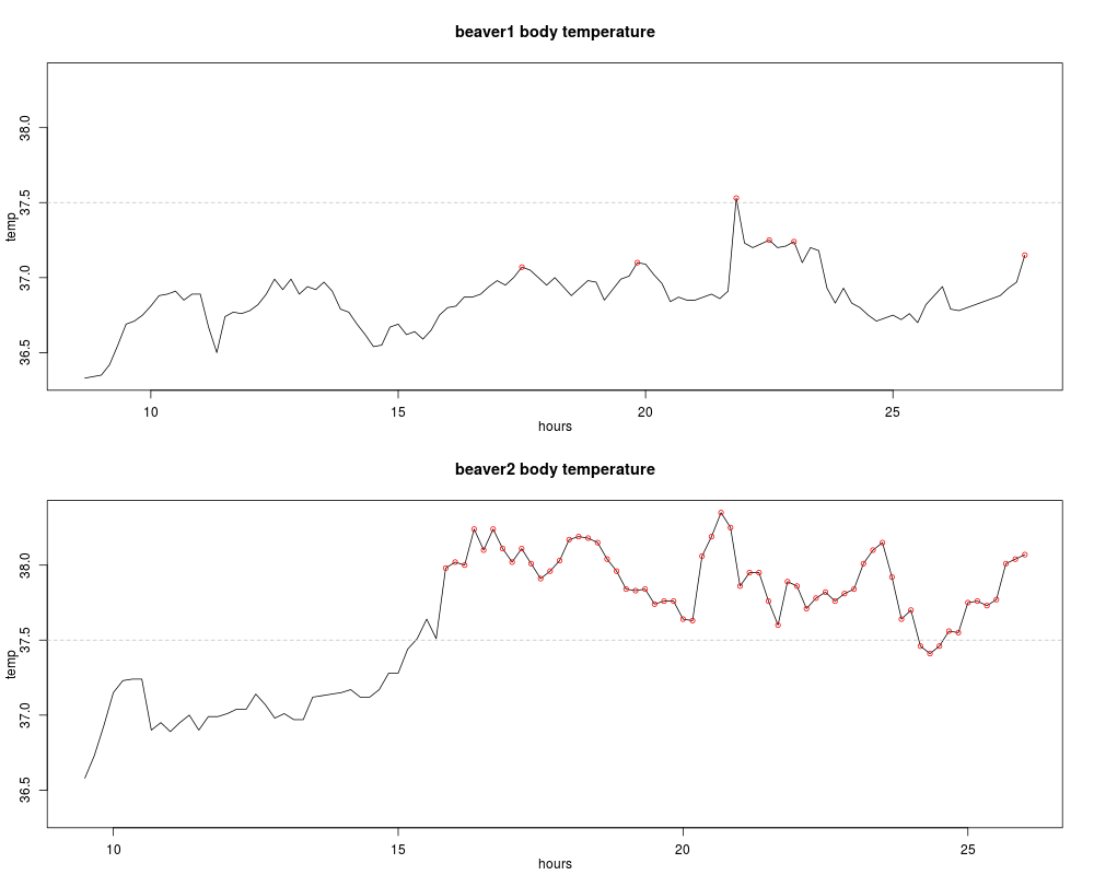
Body Temperature Series of Two Beavers

Description

Reynolds (1994) describes a small part of a study of the long-term temperature dynamics of beaver Castor canadensis in north-central Wisconsin. Body temperature was measured by telemetry every 10 minutes for four females, but data from a one period of less than a day for each of two animals is used there.

Usage

beaver1
beaver2

Format

The beaver1 data frame has 114 rows and 4 columns on body temperature measurements at 10 minute intervals.

The beaver2 data frame has 100 rows and 4 columns on body temperature measurements at 10 minute intervals.

The variables are as follows:

day

Day of observation (in days since the beginning of 1990), December 12–13 (beaver1) and November 3–4 (beaver2).

time

Time of observation, in the form 0330 for 3:30am

temp

Measured body temperature in degrees Celsius.

activ

Indicator of activity outside the retreat.

Note

The observation at 22:20 is missing in beaver1.

Source

P. S. Reynolds (1994) Time-series analyses of beaver body temperatures. Chapter 11 of Lange, N., Ryan, L., Billard, L., Brillinger, D., Conquest, L. and Greenhouse, J. eds (1994) Case Studies in Biometry. New York: John Wiley and Sons.

Examples

require(graphics)
(yl <- range(beaver1$temp, beaver2$temp))

beaver.plot <- function(bdat, ...) {
  nam <- deparse(substitute(bdat))
  with(bdat, {
    # Hours since start of day:
    hours <- time %/% 100 + 24*(day - day[1]) + (time %% 100)/60
    plot (hours, temp, type = "l", ...,
          main = paste(nam, "body temperature"))
    abline(h = 37.5, col = "gray", lty = 2)
    is.act <- activ == 1
    points(hours[is.act], temp[is.act], col = 2, cex = .8)
  })
}
op <- par(mfrow = c(2, 1), mar = c(3, 3, 4, 2), mgp = 0.9 * 2:0)
 beaver.plot(beaver1, ylim = yl)
 beaver.plot(beaver2, ylim = yl)
par(op)

Results

R version 3.3.1 (2016-06-21) -- "Bug in Your Hair"
Copyright (C) 2016 The R Foundation for Statistical Computing
Platform: x86_64-pc-linux-gnu (64-bit)

R is free software and comes with ABSOLUTELY NO WARRANTY.
You are welcome to redistribute it under certain conditions.
Type 'license()' or 'licence()' for distribution details.

R is a collaborative project with many contributors.
Type 'contributors()' for more information and
'citation()' on how to cite R or R packages in publications.

Type 'demo()' for some demos, 'help()' for on-line help, or
'help.start()' for an HTML browser interface to help.
Type 'q()' to quit R.

> library(datasets)
> png(filename="/home/ddbj/snapshot/RGM3/R_rel/result/datasets/beavers.Rd_%03d_medium.png", width=480, height=480)
> ### Name: beavers
> ### Title: Body Temperature Series of Two Beavers
> ### Aliases: beavers beaver1 beaver2
> ### Keywords: datasets
> 
> ### ** Examples
> 
> require(graphics)
> (yl <- range(beaver1$temp, beaver2$temp))
[1] 36.33 38.35
> 
> beaver.plot <- function(bdat, ...) {
+   nam <- deparse(substitute(bdat))
+   with(bdat, {
+     # Hours since start of day:
+     hours <- time %/% 100 + 24*(day - day[1]) + (time %% 100)/60
+     plot (hours, temp, type = "l", ...,
+           main = paste(nam, "body temperature"))
+     abline(h = 37.5, col = "gray", lty = 2)
+     is.act <- activ == 1
+     points(hours[is.act], temp[is.act], col = 2, cex = .8)
+   })
+ }
> op <- par(mfrow = c(2, 1), mar = c(3, 3, 4, 2), mgp = 0.9 * 2:0)
>  beaver.plot(beaver1, ylim = yl)
>  beaver.plot(beaver2, ylim = yl)
> par(op)
> 
> 
> 
> 
> 
> dev.off()
null device 
          1 
>