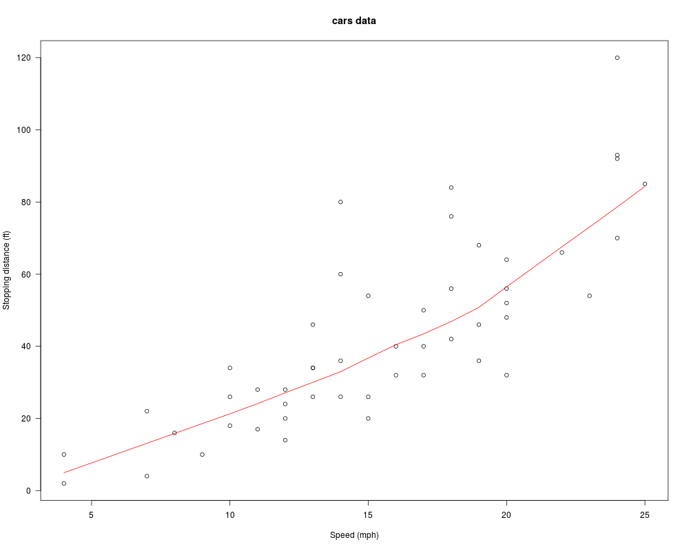
Speed and Stopping Distances of Cars

Description

The data give the speed of cars and the distances taken to stop. Note that the data were recorded in the 1920s.

Usage

cars

Format

A data frame with 50 observations on 2 variables.

Source

Ezekiel, M. (1930) Methods of Correlation Analysis. Wiley.

References

McNeil, D. R. (1977) Interactive Data Analysis. Wiley.

Examples

require(stats); require(graphics)
plot(cars, xlab = "Speed (mph)", ylab = "Stopping distance (ft)",
     las = 1)
lines(lowess(cars$speed, cars$dist, f = 2/3, iter = 3), col = "red")
title(main = "cars data")
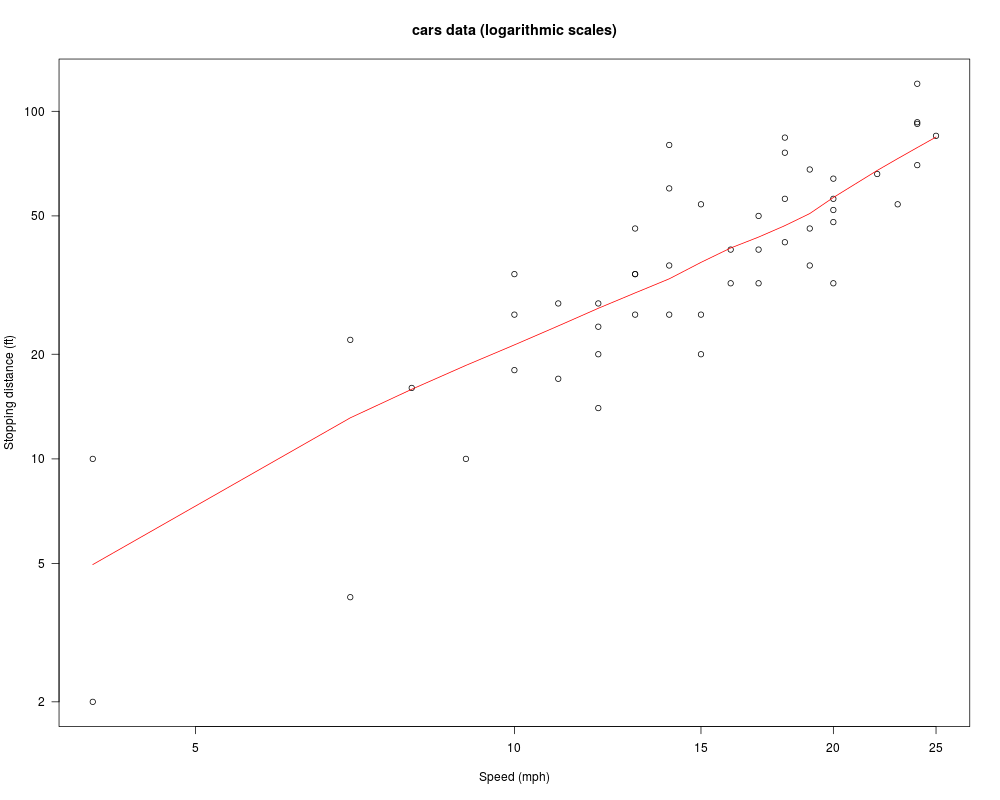
plot(cars, xlab = "Speed (mph)", ylab = "Stopping distance (ft)",
     las = 1, log = "xy")
title(main = "cars data (logarithmic scales)")
lines(lowess(cars$speed, cars$dist, f = 2/3, iter = 3), col = "red")
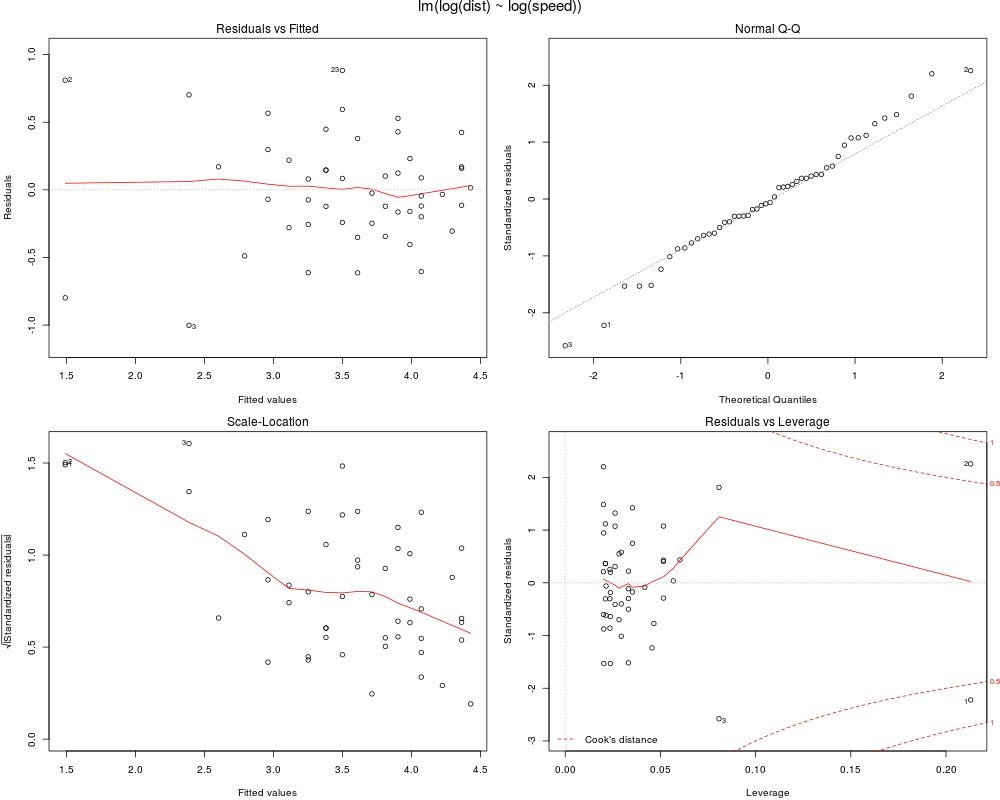
summary(fm1 <- lm(log(dist) ~ log(speed), data = cars))
opar <- par(mfrow = c(2, 2), oma = c(0, 0, 1.1, 0),
            mar = c(4.1, 4.1, 2.1, 1.1))
plot(fm1)
par(opar)

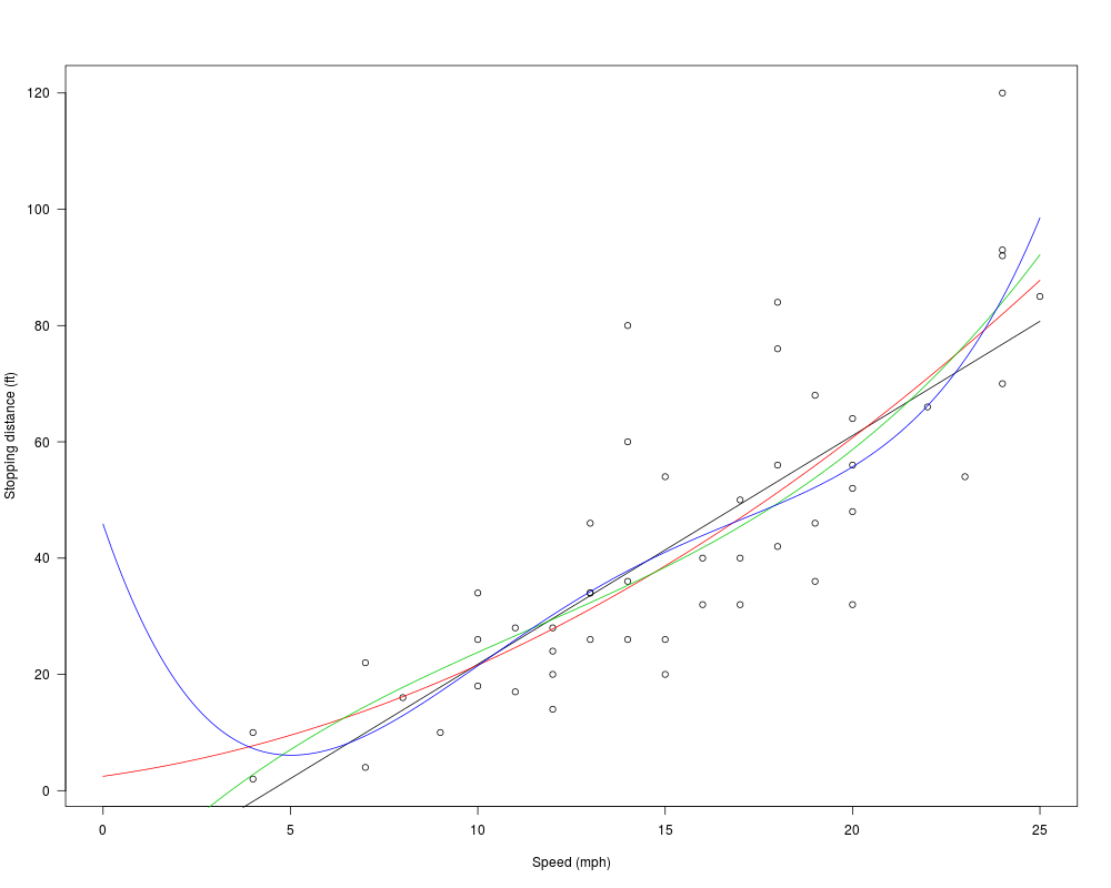
## An example of polynomial regression
plot(cars, xlab = "Speed (mph)", ylab = "Stopping distance (ft)",
    las = 1, xlim = c(0, 25))
d <- seq(0, 25, length.out = 200)
for(degree in 1:4) {
  fm <- lm(dist ~ poly(speed, degree), data = cars)
  assign(paste("cars", degree, sep = "."), fm)
  lines(d, predict(fm, data.frame(speed = d)), col = degree)
}
anova(cars.1, cars.2, cars.3, cars.4)

Results

R version 3.3.1 (2016-06-21) -- "Bug in Your Hair"
Copyright (C) 2016 The R Foundation for Statistical Computing
Platform: x86_64-pc-linux-gnu (64-bit)

R is free software and comes with ABSOLUTELY NO WARRANTY.
You are welcome to redistribute it under certain conditions.
Type 'license()' or 'licence()' for distribution details.

R is a collaborative project with many contributors.
Type 'contributors()' for more information and
'citation()' on how to cite R or R packages in publications.

Type 'demo()' for some demos, 'help()' for on-line help, or
'help.start()' for an HTML browser interface to help.
Type 'q()' to quit R.

> library(datasets)
> png(filename="/home/ddbj/snapshot/RGM3/R_rel/result/datasets/cars.Rd_%03d_medium.png", width=480, height=480)
> ### Name: cars
> ### Title: Speed and Stopping Distances of Cars
> ### Aliases: cars
> ### Keywords: datasets
> 
> ### ** Examples
> 
> require(stats); require(graphics)
> plot(cars, xlab = "Speed (mph)", ylab = "Stopping distance (ft)",
+      las = 1)
> lines(lowess(cars$speed, cars$dist, f = 2/3, iter = 3), col = "red")
> title(main = "cars data")
> plot(cars, xlab = "Speed (mph)", ylab = "Stopping distance (ft)",
+      las = 1, log = "xy")
> title(main = "cars data (logarithmic scales)")
> lines(lowess(cars$speed, cars$dist, f = 2/3, iter = 3), col = "red")
> summary(fm1 <- lm(log(dist) ~ log(speed), data = cars))

Call:
lm(formula = log(dist) ~ log(speed), data = cars)

Residuals:
     Min       1Q   Median       3Q      Max 
-1.00215 -0.24578 -0.02898  0.20717  0.88289 

Coefficients:
            Estimate Std. Error t value Pr(>|t|)    
(Intercept)  -0.7297     0.3758  -1.941   0.0581 .  
log(speed)    1.6024     0.1395  11.484 2.26e-15 ***
---
Signif. codes:  0 '***' 0.001 '**' 0.01 '*' 0.05 '.' 0.1 ' ' 1

Residual standard error: 0.4053 on 48 degrees of freedom
Multiple R-squared:  0.7331,	Adjusted R-squared:  0.7276 
F-statistic: 131.9 on 1 and 48 DF,  p-value: 2.259e-15

> opar <- par(mfrow = c(2, 2), oma = c(0, 0, 1.1, 0),
+             mar = c(4.1, 4.1, 2.1, 1.1))
> plot(fm1)
> par(opar)
> 
> ## An example of polynomial regression
> plot(cars, xlab = "Speed (mph)", ylab = "Stopping distance (ft)",
+     las = 1, xlim = c(0, 25))
> d <- seq(0, 25, length.out = 200)
> for(degree in 1:4) {
+   fm <- lm(dist ~ poly(speed, degree), data = cars)
+   assign(paste("cars", degree, sep = "."), fm)
+   lines(d, predict(fm, data.frame(speed = d)), col = degree)
+ }
> anova(cars.1, cars.2, cars.3, cars.4)
Analysis of Variance Table

Model 1: dist ~ poly(speed, degree)
Model 2: dist ~ poly(speed, degree)
Model 3: dist ~ poly(speed, degree)
Model 4: dist ~ poly(speed, degree)
  Res.Df   RSS Df Sum of Sq      F Pr(>F)
1     48 11354                           
2     47 10825  1    528.81 2.3108 0.1355
3     46 10634  1    190.35 0.8318 0.3666
4     45 10298  1    336.55 1.4707 0.2316
> 
> 
> 
> 
> 
> dev.off()
null device 
          1 
>