Carbon Dioxide Uptake in Grass Plants

Description

The CO2 data frame has 84 rows and 5 columns of data from an experiment on the cold tolerance of the grass species Echinochloa crus-galli.

Usage

CO2

Format

An object of class c("nfnGroupedData", "nfGroupedData", "groupedData", "data.frame") containing the following columns:

Plant

an ordered factor with levels Qn1 < Qn2 < Qn3 < ... < Mc1 giving a unique identifier for each plant.

Type

a factor with levels Quebec Mississippi giving the origin of the plant

Treatment

a factor with levels nonchilled chilled

conc

a numeric vector of ambient carbon dioxide concentrations (mL/L).

uptake

a numeric vector of carbon dioxide uptake rates (umol/m^2 sec).

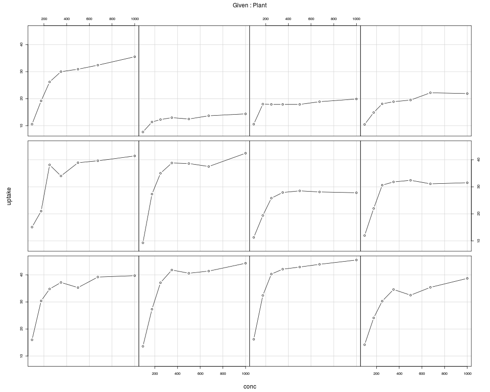
Details

The CO2 uptake of six plants from Quebec and six plants from Mississippi was measured at several levels of ambient CO2 concentration. Half the plants of each type were chilled overnight before the experiment was conducted.

This dataset was originally part of package nlme, and that has methods (including for [, as.data.frame, plot and print) for its grouped-data classes.

Source

Potvin, C., Lechowicz, M. J. and Tardif, S. (1990) “The statistical analysis of ecophysiological response curves obtained from experiments involving repeated measures”, Ecology, 71, 1389–1400.

Pinheiro, J. C. and Bates, D. M. (2000) Mixed-effects Models in S and S-PLUS, Springer.

Examples

require(stats); require(graphics)

coplot(uptake ~ conc | Plant, data = CO2, show.given = FALSE, type = "b")
## fit the data for the first plant
fm1 <- nls(uptake ~ SSasymp(conc, Asym, lrc, c0),
   data = CO2, subset = Plant == "Qn1")
summary(fm1)
## fit each plant separately
fmlist <- list()
for (pp in levels(CO2$Plant)) {
  fmlist[[pp]] <- nls(uptake ~ SSasymp(conc, Asym, lrc, c0),
      data = CO2, subset = Plant == pp)
}
## check the coefficients by plant
print(sapply(fmlist, coef), digits = 3)

Results

R version 3.3.1 (2016-06-21) -- "Bug in Your Hair"
Copyright (C) 2016 The R Foundation for Statistical Computing
Platform: x86_64-pc-linux-gnu (64-bit)

R is free software and comes with ABSOLUTELY NO WARRANTY.
You are welcome to redistribute it under certain conditions.
Type 'license()' or 'licence()' for distribution details.

R is a collaborative project with many contributors.
Type 'contributors()' for more information and
'citation()' on how to cite R or R packages in publications.

Type 'demo()' for some demos, 'help()' for on-line help, or
'help.start()' for an HTML browser interface to help.
Type 'q()' to quit R.

> library(datasets)
> png(filename="/home/ddbj/snapshot/RGM3/R_rel/result/datasets/zCO2.Rd_%03d_medium.png", width=480, height=480)
> ### Name: CO2
> ### Title: Carbon Dioxide Uptake in Grass Plants
> ### Aliases: CO2
> ### Keywords: datasets
> 
> ### ** Examples
> 
> require(stats); require(graphics)
> ## Don't show: 
> options(show.nls.convergence=FALSE)
> ## End(Don't show)
> coplot(uptake ~ conc | Plant, data = CO2, show.given = FALSE, type = "b")
> ## fit the data for the first plant
> fm1 <- nls(uptake ~ SSasymp(conc, Asym, lrc, c0),
+    data = CO2, subset = Plant == "Qn1")
> summary(fm1)

Formula: uptake ~ SSasymp(conc, Asym, lrc, c0)

Parameters:
     Estimate Std. Error t value Pr(>|t|)    
Asym  38.1398     0.9164  41.620 1.99e-06 ***
lrc  -34.2766    18.9661  -1.807    0.145    
c0    -4.3806     0.2042 -21.457 2.79e-05 ***
---
Signif. codes:  0 '***' 0.001 '**' 0.01 '*' 0.05 '.' 0.1 ' ' 1

Residual standard error: 1.663 on 4 degrees of freedom

> ## fit each plant separately
> fmlist <- list()
> for (pp in levels(CO2$Plant)) {
+   fmlist[[pp]] <- nls(uptake ~ SSasymp(conc, Asym, lrc, c0),
+       data = CO2, subset = Plant == pp)
+ }
> ## check the coefficients by plant
> print(sapply(fmlist, coef), digits = 3)
        Qn1    Qn2    Qn3   Qc1    Qc3    Qc2    Mn3    Mn2   Mn1   Mc2     Mc3
Asym  38.14  42.87  44.23 36.43  40.68  39.82  28.48  32.13 34.08 13.56   18.54
lrc  -34.28 -29.66 -37.63 -9.90 -11.54 -51.53 -17.37 -29.04 -8.81 -1.98 -136.11
c0    -4.38  -4.67  -4.49 -4.86  -4.95  -4.46  -4.59  -4.47 -5.06 -4.56   -3.47
       Mc1
Asym 21.79
lrc   2.45
c0   -5.14
> 
> 
> 
> 
> 
> dev.off()
null device 
          1 
>